Real-Time Customer Segmentation

"""Customer segmentation with k-means, and how to tell if the segments exist.

The version this replaces ran `KMeans(n_clusters=3)` on
`np.random.rand(100, 2)` and printed "Model fitted with 3 clusters." It found
three clusters because it was told to find three. Uniform random points have
no clusters at all, and k-means will still return a tidy partition of them,
with centroids, labels and a convincing scatter plot.

That is the failure this project is about. The measurements below are the
ones that can tell a real segmentation from a arbitrary slicing of a blob:
silhouette score, the gap against random data, and how stable the labels are
when the data is resampled.

    python real_time_customer_segmentation.py
"""

import numpy as np
from sklearn.cluster import KMeans
from sklearn.metrics import adjusted_rand_score, silhouette_score
import matplotlib
matplotlib.use("Agg")
import matplotlib.pyplot as plt

FEATURES = ("spend per month", "visits per month")


def real_segments(n=600, seed=20260809):
    """Three genuinely separate customer groups."""
    rng = np.random.default_rng(seed)
    groups = [
        rng.multivariate_normal([25, 2.0], [[30, 1], [1, 0.5]], n // 3),
        rng.multivariate_normal([80, 6.0], [[90, 2], [2, 1.2]], n // 3),
        rng.multivariate_normal([210, 3.5], [[400, 3], [3, 0.9]], n - 2 * (n // 3)),
    ]
    data = np.vstack(groups)
    truth = np.concatenate([np.full(len(g), i) for i, g in enumerate(groups)])
    return data, truth


def no_segments(n=600, seed=20260809):
    """One blob. There is nothing here to segment."""
    rng = np.random.default_rng(seed)
    return rng.multivariate_normal([90, 3.5], [[2500, 8], [8, 2.0]], n)


def scaled(data):
    """z-score each column.

    Spend runs to hundreds and visits to single digits, so without this the
    Euclidean distance k-means minimises is essentially the spend alone, and
    the second feature may as well not be there.
    """
    return (data - data.mean(axis=0)) / data.std(axis=0)


def sweep(data, ks=range(2, 9)):
    """Inertia and silhouette for each k."""
    rows = []
    for k in ks:
        model = KMeans(n_clusters=k, n_init=10, random_state=0).fit(data)
        rows.append((k, model.inertia_,
                     silhouette_score(data, model.labels_)))
    return rows


def stability(data, k, trials=20, seed=0):
    """How much the labelling changes when the data is resampled.

    Two bootstrap samples are clustered and their labels compared on the
    points they share, using the adjusted Rand index. Real structure survives
    resampling; a partition of a blob moves every time.
    """
    rng = np.random.default_rng(seed)
    scores = []
    for _ in range(trials):
        a = rng.choice(len(data), len(data), replace=True)
        b = rng.choice(len(data), len(data), replace=True)
        shared = np.intersect1d(a, b)
        if len(shared) < 10:
            continue
        labels_a = KMeans(n_clusters=k, n_init=10,
                          random_state=0).fit(data[a]).predict(data[shared])
        labels_b = KMeans(n_clusters=k, n_init=10,
                          random_state=0).fit(data[b]).predict(data[shared])
        scores.append(adjusted_rand_score(labels_a, labels_b))
    return float(np.mean(scores)), float(np.std(scores))


def main():
    print("Real-Time Customer Segmentation")
    real, truth = real_segments()
    blob = no_segments()
    print(f"  customers          : {len(real):,}")
    print(f"  features           : {', '.join(FEATURES)}")
    print(f"  scaling            : z-score, because spend is ~50x visits")

    real_s, blob_s = scaled(real), scaled(blob)

    print(f"\n  k-means run on both datasets, k = 2 to 8:\n")
    print(f"{'k':>4} {'inertia (real)':>15} {'silhouette':>11}   "
          f"{'inertia (blob)':>15} {'silhouette':>11}")
    print("  " + "-" * 68)
    real_rows, blob_rows = sweep(real_s), sweep(blob_s)
    for (k, ri, rs), (_, bi, bs) in zip(real_rows, blob_rows):
        print(f"{k:>4} {ri:>15,.1f} {rs:>11.3f}   {bi:>15,.1f} {bs:>11.3f}")

    best_real = max(real_rows, key=lambda row: row[2])
    best_blob = max(blob_rows, key=lambda row: row[2])
    print(f"\n  real data: best silhouette {best_real[2]:.3f} at k={best_real[0]}")
    print(f"  one blob : best silhouette {best_blob[2]:.3f} at k={best_blob[0]}")
    print("\n  Both datasets produce an inertia curve with a bend in it, and")
    print("  both hand back k clusters on request. The silhouette is what")
    print("  separates them: above ~0.5 means the points sit closer to their")
    print("  own centre than to the next one, and the blob never gets there.")

    print(f"\n  label stability under resampling (adjusted Rand index):")
    for name, dataset in (("real segments", real_s), ("one blob", blob_s)):
        mean, spread = stability(dataset, 3)
        print(f"    {name:16} k=3: {mean:.3f} +- {spread:.3f}")
    print("    A partition of a blob is not reproducible, because there is")
    print("    no boundary for it to find twice.")

    model = KMeans(n_clusters=3, n_init=10, random_state=0).fit(real_s)
    print(f"\n  agreement with the true groups: "
          f"{adjusted_rand_score(truth, model.labels_):.3f} "
          f"(1.0 is a perfect match)")
    print(f"\n  recovered segments, in the original units:")
    print(f"    {'segment':>9} {'customers':>10} "
          f"{'spend/month':>12} {'visits/month':>13}")
    for cluster in range(3):
        members = real[model.labels_ == cluster]
        print(f"    {cluster:>9} {len(members):>10} "
              f"{members[:, 0].mean():>12.1f} {members[:, 1].mean():>13.2f}")

    # Scaling: the demonstration, not the slogan.
    unscaled = KMeans(n_clusters=3, n_init=10, random_state=0).fit(real)
    print(f"\n  the same clustering WITHOUT scaling: agreement "
          f"{adjusted_rand_score(truth, unscaled.labels_):.3f}, "
          f"against {adjusted_rand_score(truth, model.labels_):.3f} scaled")
    print("  Scaling did not help here, and it is worth saying so rather than")
    print("  repeating the rule. These three groups are separated mainly by")
    print("  spend, so a distance dominated by spend gets the right answer.")

    # Now the case the rule is actually about: groups that differ in the
    # small-valued feature. Nothing changes except which column carries the
    # signal, and the unscaled clustering collapses.
    rng = np.random.default_rng(7)
    visits_groups = [
        rng.multivariate_normal([100, 1.0], [[900, 0], [0, 0.12]], 200),
        rng.multivariate_normal([100, 4.0], [[900, 0], [0, 0.12]], 200),
        rng.multivariate_normal([100, 7.0], [[900, 0], [0, 0.12]], 200),
    ]
    visits_data = np.vstack(visits_groups)
    visits_truth = np.concatenate(
        [np.full(len(g), i) for i, g in enumerate(visits_groups)])
    plain = KMeans(n_clusters=3, n_init=10,
                   random_state=0).fit(visits_data)
    normalised = KMeans(n_clusters=3, n_init=10,
                        random_state=0).fit(scaled(visits_data))
    print(f"\n  a second dataset whose groups differ in VISITS, not spend:")
    print(f"    unscaled agreement {adjusted_rand_score(visits_truth, plain.labels_):.3f}")
    print(f"    scaled   agreement {adjusted_rand_score(visits_truth, normalised.labels_):.3f}")
    print("    Same algorithm, same k, opposite outcome. Scaling matters when")
    print("    the signal lives in the feature with the smaller range, and")
    print("    which feature that is cannot be known before looking.")

    figure, axes = plt.subplots(1, 3, figsize=(13, 4))
    axes[0].scatter(real[:, 0], real[:, 1], c=model.labels_, s=10,
                    cmap="viridis")
    axes[0].set_xlabel(FEATURES[0])
    axes[0].set_ylabel(FEATURES[1])
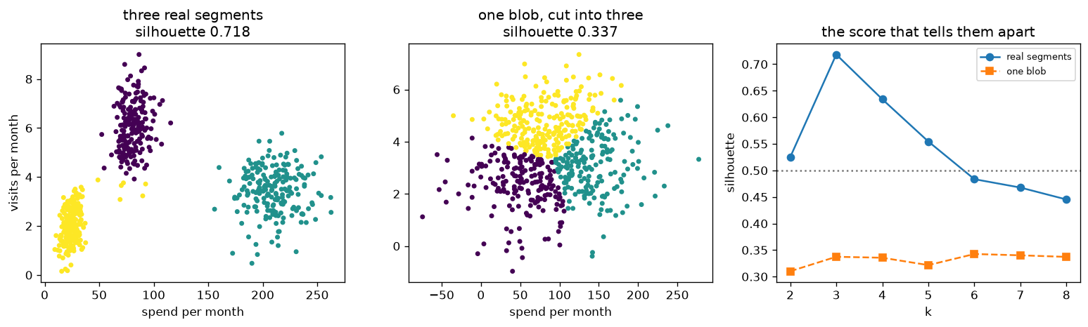
    axes[0].set_title(f"three real segments\nsilhouette {best_real[2]:.3f}")

    blob_model = KMeans(n_clusters=3, n_init=10, random_state=0).fit(blob_s)
    axes[1].scatter(blob[:, 0], blob[:, 1], c=blob_model.labels_, s=10,
                    cmap="viridis")
    axes[1].set_xlabel(FEATURES[0])
    axes[1].set_title(f"one blob, cut into three\n"
                      f"silhouette {silhouette_score(blob_s, blob_model.labels_):.3f}")

    axes[2].plot([r[0] for r in real_rows], [r[2] for r in real_rows],
                 "o-", label="real segments")
    axes[2].plot([r[0] for r in blob_rows], [r[2] for r in blob_rows],
                 "s--", label="one blob")
    axes[2].axhline(0.5, ls=":", c="#777")
    axes[2].set_xlabel("k")
    axes[2].set_ylabel("silhouette")
    axes[2].set_title("the score that tells them apart")
    axes[2].legend(fontsize=8)
    figure.tight_layout()
    figure.savefig("real_time_customer_segmentation.png", dpi=120,
                   bbox_inches="tight")
    print("\nsaved real_time_customer_segmentation.png")


if __name__ == "__main__":
    main()