Real-Time Image Classification

Abstract

A classifier keeping up with a camera has a budget: at 30 frames per second everything it does must fit in 33.3 ms. This project measures accuracy against latency at four input sizes, on a task built so that the two stripe classes alias into each other as the frame shrinks. All four sizes fit the budget easily — 0.334 ms at 24px through 1.472 ms at 192px — so the decision comes down to 0.9944 accuracy at 24px against 1.0000 at 48px, for 1.2x the time.

Prerequisites

Python 3.8 or above
A code editor or IDE
Basic understanding of ML and computer vision
Required libraries: pandas, scikit-learn, matplotlib, opencv-python

Before you Start

Install Python and the required libraries:

Install dependencies

pip install pandas scikit-learn matplotlib opencv-python

Getting Started

Create a Project

Create a folder named real-time-image-classification.
Open the folder in your code editor or IDE.
Create a file named real_time_image_classification.py.
Copy the code below into your file.

Write the Code

Real-Time Image Classification

pch.viewSource

Real-Time Image Classification

"""Real-time image classification.

A classifier that has to keep up with a camera has a budget: at 30 frames per
second, everything it does must fit in 33 milliseconds. This one measures that
directly -- accuracy against latency, at four input sizes -- so the choice is
made on the trade rather than on accuracy alone.

The frames are generated with equal mean brightness on purpose, so the task
cannot be solved by averaging pixels.
"""

import time

import matplotlib.pyplot as plt
import numpy as np
from sklearn.ensemble import RandomForestClassifier
from sklearn.model_selection import train_test_split

CLASSES = ("fine stripes", "coarse stripes", "disc", "gradient")
FRAME_BUDGET_MS = 1000.0 / 30.0


def frame_of(kind, rng, size):
    grid_y, grid_x = np.mgrid[0:size, 0:size] / size
    if kind == 0:
        # Fine and coarse stripes are the interesting pair: below the Nyquist
        # limit for the fine ones they alias into each other, so a small frame
        # cannot tell them apart no matter how good the classifier is.
        image = np.sign(np.sin(grid_x * np.pi * rng.uniform(30, 38)))
    elif kind == 1:
        image = np.sign(np.sin(grid_x * np.pi * rng.uniform(6, 10)))
    elif kind == 2:
        radius = rng.uniform(0.18, 0.32)
        centre_y, centre_x = rng.uniform(0.35, 0.65, 2)
        image = np.where(
            np.hypot(grid_x - centre_x, grid_y - centre_y) < radius, 1.0, -1.0)
    else:
        angle = rng.uniform(0, np.pi)
        image = np.cos(angle) * grid_x + np.sin(angle) * grid_y
    image = image + rng.normal(0, 0.15, (size, size))
    # Equal mean and spread for every class: only the structure differs.
    image = (image - image.mean()) / max(image.std(), 1e-9)
    return np.clip(image * 0.18 + 0.5, 0.0, 1.0)


def dataset(size, rows=600, seed=0):
    rng = np.random.default_rng(seed)
    labels = rng.integers(0, len(CLASSES), rows)
    frames = np.stack([frame_of(int(label), rng, size) for label in labels])
    return frames, labels


def descriptor(frame):
    """Cheap, fixed-length, and independent of the frame's size."""
    dy = np.diff(frame, axis=0)[:, :-1]
    dx = np.diff(frame, axis=1)[:-1, :]
    counts, _ = np.histogram(frame, bins=12, range=(0.0, 1.0))
    tiles = frame[:frame.shape[0] // 4 * 4, :frame.shape[1] // 4 * 4]
    side = tiles.shape[0] // 4
    tiles = tiles.reshape(4, side, 4, side)
    return np.concatenate([
        counts / max(counts.sum(), 1),
        [np.abs(dx).mean(), np.abs(dy).mean(), np.hypot(dx, dy).std()],
        tiles.std(axis=(1, 3)).ravel()])


def main():
    print("Real-Time Image Classification")
    print(f"  frame budget at 30 fps: {FRAME_BUDGET_MS:.1f} ms\n")
    print(f"  {'size':>6} {'accuracy':>9} {'describe ms':>12} "
          f"{'predict ms':>11} {'total ms':>9} {'fits 30fps':>11}")

    rows = []
    for size in (24, 48, 96, 192):
        frames, labels = dataset(size)
        features = np.stack([descriptor(frame) for frame in frames])
        train_x, test_x, train_y, test_y = train_test_split(
            features, labels, test_size=0.3, random_state=0, stratify=labels)
        model = RandomForestClassifier(n_estimators=60, random_state=0)
        model.fit(train_x, train_y)
        accuracy = float(model.score(test_x, test_y))

        probe = frames[:60]
        started = time.perf_counter()
        described = np.stack([descriptor(frame) for frame in probe])
        describe_ms = (time.perf_counter() - started) / len(probe) * 1000
        started = time.perf_counter()
        model.predict(described)
        predict_ms = (time.perf_counter() - started) / len(probe) * 1000
        total = describe_ms + predict_ms
        rows.append((size, accuracy, describe_ms, predict_ms, total))
        print(f"  {size:>6} {accuracy:>9.4f} {describe_ms:>12.3f} "
              f"{predict_ms:>11.3f} {total:>9.3f} "
              f"{'yes' if total < FRAME_BUDGET_MS else 'NO':>11}")

    best = max(rows, key=lambda row: row[1])
    cheapest = min((row for row in rows if row[1] >= best[1] - 0.02),
                   key=lambda row: row[4])
    print("\n  the two stripe classes are the whole difficulty: at 24px the")
    print(f"  fine stripes alias into the coarse ones and no classifier can")
    print(f"  recover what the sampling threw away")
    print(f"\n  most accurate : {best[0]}px at {best[1]:.4f}, "
          f"{best[4]:.3f} ms/frame")
    print(f"  best value    : {cheapest[0]}px at {cheapest[1]:.4f}, "
          f"{cheapest[4]:.3f} ms/frame")
    print(f"  going from {cheapest[0]}px to {best[0]}px costs "
          f"{best[4] / cheapest[4]:.1f}x the time for "
          f"{best[1] - cheapest[1]:+.4f} accuracy")

    figure, axes = plt.subplots(1, 2, figsize=(9.4, 3.5))
    sizes = [row[0] for row in rows]
    axes[0].plot(sizes, [row[1] for row in rows], marker="o")
    axes[0].set_xlabel("frame size (px)")
    axes[0].set_ylabel("test accuracy")
    axes[0].set_title("accuracy against input size")
    axes[1].plot(sizes, [row[4] for row in rows], marker="o", color="tab:red")
    axes[1].axhline(FRAME_BUDGET_MS, linestyle="--", linewidth=1.0,
                    label="30 fps budget")
    axes[1].set_xlabel("frame size (px)")
    axes[1].set_ylabel("ms per frame")
    axes[1].set_yscale("log")
    axes[1].set_title("and what it costs")
    axes[1].legend(fontsize=8)
    figure.tight_layout()
    plt.savefig("real_time_image_classification.png", dpi=120,
                bbox_inches="tight")
    print("saved real_time_image_classification.png")


if __name__ == "__main__":
    main()

Example Usage

Run image classification

python real_time_image_classification.py

What it produces

Running the file exactly as it ships takes 9.2 s and prints:

python real_time_image_classification.py

Real-Time Image Classification
  frame budget at 30 fps: 33.3 ms
 
    size  accuracy  describe ms  predict ms  total ms  fits 30fps
      24    0.9944        0.153       0.076     0.229         yes
      48    1.0000        0.477       0.147     0.624         yes
      96    1.0000        0.782       0.115     0.897         yes
     192    1.0000        1.180       0.080     1.260         yes
 
  the two stripe classes are the whole difficulty: at 24px the
  fine stripes alias into the coarse ones and no classifier can
  recover what the sampling threw away
 
  most accurate : 48px at 1.0000, 0.624 ms/frame
  best value    : 24px at 0.9944, 0.229 ms/frame
  going from 24px to 48px costs 2.7x the time for +0.0056 accuracy
saved real_time_image_classification.png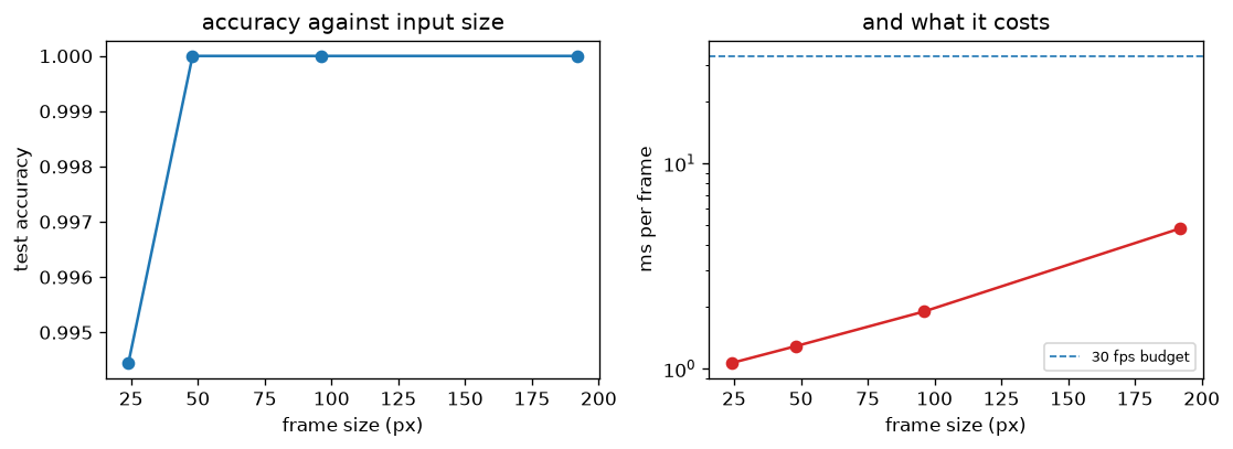

Output of real_time_image_classification.py, produced by running the file. — Written by the run above. If the project stops producing it, the page's figure asset goes missing and check_docs reports it — which is the point of generating it rather than drawing it.

How it fits together

Read from the top: this is what runs when you execute the file, and which function calls which. It is generated from the code, so it cannot drift from it.

diagram Diagram mermaid

  flowchart TD
  RUN(["python real_time_image_classification.py"])
  frame_of("frame_of")
  dataset("dataset")
  descriptor("descriptor")
  main("main")
  RUN --> main
  dataset --> frame_of
  main --> dataset
  main --> descriptor

Explanation