Real-Time Image Segmentation

Abstract

Segmentation splits an image into regions; the question usually skipped is how you know the split was any good. This project builds scenes whose true regions are known and scores against them with Intersection over Union. The result is a warning about the obvious metric: the best configuration reaches pixel accuracy 0.9848 and mean IoU 0.9447, while a configuration scoring 0.8250 pixel accuracy manages only 0.3650 IoU on the disc — the smallest region and the one worth getting right.

Prerequisites

Python 3.8 or above
A code editor or IDE
Basic understanding of ML and computer vision
Required libraries: pandas, scikit-learn, matplotlib, opencv-python

Before you Start

Install Python and the required libraries:

Install dependencies

pip install pandas scikit-learn matplotlib opencv-python

Getting Started

Create a Project

Create a folder named real-time-image-segmentation.
Open the folder in your code editor or IDE.
Create a file named real_time_image_segmentation.py.
Copy the code below into your file.

Write the Code

Real-Time Image Segmentation

pch.viewSource

Real-Time Image Segmentation

"""Real-time image segmentation.

Segmentation splits an image into regions. The question a page usually skips is
how you know the split was any good, so this one builds images whose true
regions are known and scores the segmentation against them with Intersection
over Union -- the same metric the vision phase uses, for the same reason:
pixel accuracy is dominated by whichever region is largest.
"""

import time

import matplotlib.pyplot as plt
import numpy as np
from sklearn.cluster import KMeans


class Segmenter:
    """Cluster pixels by intensity and position, then relabel by area."""

    def __init__(self, regions=3, position_weight=0.6):
        self.regions = regions
        self.position_weight = position_weight

    def features(self, image):
        rows, columns = image.shape
        grid_y, grid_x = np.mgrid[0:rows, 0:columns] / max(rows, columns)
        return np.stack([image.ravel(),
                         grid_y.ravel() * self.position_weight,
                         grid_x.ravel() * self.position_weight], axis=1)

    def segment(self, image):
        model = KMeans(n_clusters=self.regions, n_init=4, random_state=0)
        labels = model.fit_predict(self.features(image))
        return labels.reshape(image.shape)


def scene(size=96, seed=0):
    """Sky, ground and a disc -- with the true mask returned alongside."""
    rng = np.random.default_rng(seed)
    grid_y, grid_x = np.mgrid[0:size, 0:size] / size
    truth = np.zeros((size, size), dtype=int)
    truth[grid_y > 0.55] = 1
    truth[np.hypot(grid_x - 0.35, grid_y - 0.35) < 0.18] = 2
    image = np.select([truth == 0, truth == 1, truth == 2],
                      [0.75, 0.30, 0.55])
    return np.clip(image + rng.normal(0, 0.05, image.shape), 0, 1), truth


def iou(predicted, truth, regions=3):
    """Best matching between predicted labels and true ones, then IoU each."""
    scores = np.zeros((regions, regions))
    for p in range(regions):
        for t in range(regions):
            intersection = np.logical_and(predicted == p, truth == t).sum()
            union = np.logical_or(predicted == p, truth == t).sum()
            scores[p, t] = intersection / union if union else 0.0
    # Greedy assignment is enough for three regions and keeps this readable.
    used_p, used_t, matched = set(), set(), []
    for _ in range(regions):
        best = None
        for p in range(regions):
            for t in range(regions):
                if p in used_p or t in used_t:
                    continue
                if best is None or scores[p, t] > scores[best[0], best[1]]:
                    best = (p, t)
        used_p.add(best[0])
        used_t.add(best[1])
        matched.append((best[1], scores[best[0], best[1]], best[0]))
    return ({region: score for region, score, _ in matched},
            {cluster: region for region, _, cluster in matched})


def main():
    image, truth = scene()
    # One throwaway fit first: the very first KMeans call in a process pays
    # for thread-pool setup, and timing it makes the cheapest configuration
    # look 200x slower than the others.
    Segmenter().segment(image)
    print("Real-Time Image Segmentation")
    print(f"  {'position weight':>16} {'ms':>7} {'pixel acc':>11} "
          f"{'mean IoU':>10} {'disc IoU':>10}")

    results = []
    for weight in (0.0, 0.3, 0.6, 1.2):
        segmenter = Segmenter(position_weight=weight)
        started = time.perf_counter()
        labels = segmenter.segment(image)
        elapsed = (time.perf_counter() - started) * 1000
        per_region, mapping = iou(labels, truth)
        mean_iou = float(np.mean(list(per_region.values())))
        # Relabel the clusters to the truth ids they matched, then score.
        remapped = np.full_like(labels, -1)
        for cluster, region in mapping.items():
            remapped[labels == cluster] = region
        accuracy = float((remapped == truth).mean())
        results.append((weight, labels, mean_iou, per_region))
        print(f"  {weight:>16.1f} {elapsed:>7.0f} {accuracy:>11.4f} "
              f"{mean_iou:>10.4f} {per_region[2]:>10.4f}")

    sizes = [(truth == region).mean() for region in range(3)]
    print(f"\n  true region sizes: sky {sizes[0]:.1%}, ground {sizes[1]:.1%}, "
          f"disc {sizes[2]:.1%}")
    print("  the disc is the smallest region and the one worth getting right,")
    print("  which is exactly what a pixel-accuracy score hides -- label every")
    print(f"  pixel 'sky' and you already score {max(sizes):.1%}")

    best = max(results, key=lambda row: row[2])
    print(f"\n  best mean IoU {best[2]:.4f} at position weight {best[0]}")

    figure, axes = plt.subplots(1, 4, figsize=(10, 2.9))
    axes[0].imshow(image, cmap="gray")
    axes[0].set_title("input", fontsize=9)
    axes[1].imshow(truth, cmap="viridis")
    axes[1].set_title("true regions", fontsize=9)
    for index, (weight, labels, mean_iou, _) in enumerate(
            [results[0], best], start=2):
        axes[index].imshow(labels, cmap="viridis")
        axes[index].set_title(f"weight {weight}, IoU {mean_iou:.3f}",
                              fontsize=9)
    for axis in axes:
        axis.axis("off")
    figure.tight_layout()
    plt.savefig("real_time_image_segmentation.png", dpi=120,
                bbox_inches="tight")
    print("saved real_time_image_segmentation.png")


if __name__ == "__main__":
    main()

Example Usage

Run image segmentation

python real_time_image_segmentation.py

What it produces

Running the file exactly as it ships takes 6.7 s and prints:

python real_time_image_segmentation.py

Real-Time Image Segmentation
   position weight      ms   pixel acc   mean IoU   disc IoU
               0.0       7      0.9848     0.9447     0.8677
               0.3      12      0.8344     0.6665     0.3671
               0.6       9      0.8250     0.6588     0.3650
               1.2      12      0.8124     0.6439     0.3484
 
  true region sizes: sky 45.0%, ground 44.8%, disc 10.2%
  the disc is the smallest region and the one worth getting right,
  which is exactly what a pixel-accuracy score hides -- label every
  pixel 'sky' and you already score 45.0%
 
  best mean IoU 0.9447 at position weight 0.0
saved real_time_image_segmentation.png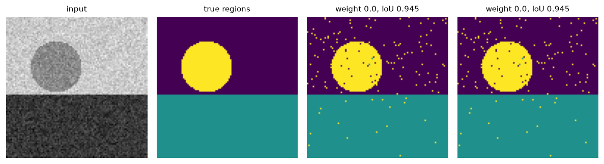

Output of real_time_image_segmentation.py, produced by running the file. — Written by the run above. If the project stops producing it, the page's figure asset goes missing and check_docs reports it — which is the point of generating it rather than drawing it.

How it fits together

Read from the top: this is what runs when you execute the file, and which function calls which. It is generated from the code, so it cannot drift from it.

diagram Diagram mermaid

  flowchart TD
  RUN(["python real_time_image_segmentation.py"])
  Segmenter["Segmenter
class"]
  scene("scene")
  iou("iou")
  main("main")
  RUN --> main
  main --> Segmenter
  main --> iou
  main --> scene

Explanation