Real-Time Sales Forecasting

Abstract

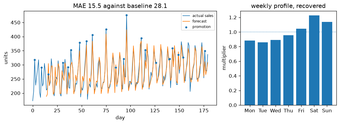
Sales are demand plus what the business does to it: a weekend lift and promotions. This project decomposes the series into level, weekly profile and promotion effect rather than fitting raw lags. It recovers the weekly shape and reaches MAE 15.5 against a same-day-last-week baseline’s 28.1, a 45.0% improvement — and shows why the obvious estimate of promotion lift is wrong by 52 units.

Prerequisites

Python 3.8 or above
A code editor or IDE
Basic understanding of ML and analytics
Required libraries: pandas, scikit-learn, matplotlib

Before you Start

Install Python and the required libraries:

Install dependencies

pip install pandas scikit-learn matplotlib

Getting Started

Create a Project

Create a folder named real-time-sales-forecasting.
Open the folder in your code editor or IDE.
Create a file named real_time_sales_forecasting.py.
Copy the code below into your file.

Write the Code

Real-Time Sales Forecasting

pch.viewSource

Real-Time Sales Forecasting

"""Real-time sales forecasting.

Sales are demand plus the things a business does to it: a weekend lift, a
promotion that pulls sales forward, and a hard floor at zero. This forecaster
decomposes the series into level, weekly profile and promotion effect rather
than fitting raw lags, and reports where each component earns its place.
"""

import matplotlib.pyplot as plt
import numpy as np

WEEK = 7


class SeasonalForecaster:
    """Level + multiplicative weekly profile + an additive promotion lift."""

    def __init__(self, window=56):
        self.window = window
        self.history = []
        self.promotions = []

    def observe(self, value, promoted):
        self.history.append(float(value))
        self.promotions.append(bool(promoted))

    def ready(self):
        return len(self.history) >= 2 * WEEK

    def _profile(self, values, start):
        """Average ratio to the local level, per day of week.

        `start` is the absolute index of `values[0]`. Without it the day-of-week
        buckets are taken from positions inside the window, which only lines up
        when the window happens to begin on a Monday -- and silently returns a
        flat, shifted profile the rest of the time.
        """
        series = np.asarray(values, dtype=float)
        level = series.mean()
        profile = np.ones(WEEK)
        days = (np.arange(len(series)) + start) % WEEK
        for day in range(WEEK):
            day_values = series[days == day]
            if len(day_values):
                profile[day] = day_values.mean() / level if level else 1.0
        return level, profile

    def _promotion_lift(self, naive=False):
        """Extra units on a promoted day.

        The obvious estimator -- mean(promoted) minus mean(everything else) --
        is confounded: promotions land on whatever weekday they land on, and a
        Saturday sells 1.35x a Monday regardless. Dividing out the weekly
        profile first removes that, and the two numbers are printed side by
        side because the gap between them is the whole point.
        """
        values = np.asarray(self.history[-self.window:], dtype=float)
        flags = np.asarray(self.promotions[-self.window:], dtype=bool)
        if not (flags.any() and (~flags).any()):
            return 0.0
        if naive:
            return float(values[flags].mean() - values[~flags].mean())
        start = len(self.history) - len(values)
        level, profile = self._profile(values, start)
        days = (np.arange(len(values)) + start) % WEEK
        expected = level * profile[days]
        residual = values - expected
        return float(residual[flags].mean() - residual[~flags].mean())

    def forecast(self, next_day_index, promoted):
        if not self.ready():
            return self.history[-1] if self.history else 0.0
        window = self.history[-self.window:]
        level, profile = self._profile(window, len(self.history) - len(window))
        base = level * profile[next_day_index % WEEK]
        if promoted:
            base += self._promotion_lift()
        return max(base, 0.0)


def sales_series(periods=180, seed=1):
    rng = np.random.default_rng(seed)
    day = np.arange(periods)
    weekly = np.array([0.86, 0.90, 0.95, 1.00, 1.15, 1.35, 1.25])
    level = 220 + 0.35 * day
    promoted = rng.random(periods) < 0.15
    values = level * weekly[day % WEEK] + promoted * 90.0
    values = values + rng.normal(0, 14.0, periods)
    return np.maximum(values, 0.0), promoted


def replay(values, promoted, forecaster):
    errors, naive_errors, predictions = [], [], []
    for index, (actual, promo) in enumerate(zip(values, promoted)):
        predicted = forecaster.forecast(index, promo)
        naive = (forecaster.history[-WEEK] if len(forecaster.history) >= WEEK
                 else (forecaster.history[-1] if forecaster.history else actual))
        if forecaster.ready():
            errors.append(abs(predicted - actual))
            naive_errors.append(abs(naive - actual))
            predictions.append((index, predicted))
        forecaster.observe(actual, promo)
    return np.asarray(errors), np.asarray(naive_errors), predictions


def main():
    values, promoted = sales_series()
    forecaster = SeasonalForecaster()
    errors, naive_errors, predictions = replay(values, promoted, forecaster)

    print("Real-Time Sales Forecasting")
    print(f"  days replayed            : {len(values)}")
    print(f"  promoted days            : {int(promoted.sum())}")
    print(f"  seasonal model MAE       : {errors.mean():.3f}")
    print(f"  same-day-last-week MAE   : {naive_errors.mean():.3f}")
    gain = (naive_errors.mean() - errors.mean()) / naive_errors.mean()
    print(f"  improvement over that    : {gain:.1%}")
    naive_lift = forecaster._promotion_lift(naive=True)
    adjusted_lift = forecaster._promotion_lift()
    print(f"  promotion lift, naive    : {naive_lift:.1f} units/day")
    print(f"  promotion lift, adjusted : {adjusted_lift:.1f} units/day "
          f"(true 90.0)")
    print(f"  naive is off by {abs(90.0 - naive_lift):.1f}, adjusted by "
          f"{abs(90.0 - adjusted_lift):.1f} -- removing the weekly profile "
          f"fixes most")
    print(f"  of the bias; the rest is that only "
          f"{int(np.asarray(forecaster.promotions[-56:]).sum())} of the last 56"
          f" days were promoted, which is a small sample")

    tail = forecaster.history[-56:]
    _, profile = forecaster._profile(tail, len(forecaster.history) - len(tail))
    names = ("Mon", "Tue", "Wed", "Thu", "Fri", "Sat", "Sun")
    print("\n  recovered weekly profile (1.00 = an average day):")
    for name, factor in zip(names, profile):
        print(f"    {name} {factor:.3f}")
    print("  the naive baseline is same-day-last-week, which already carries")
    print("  the weekly shape -- so the gain above is what decomposition adds")
    print("  ON TOP of seasonality, not the value of seasonality itself")

    steps, predicted = zip(*predictions)
    figure, axes = plt.subplots(1, 2, figsize=(9.6, 3.6),
                                width_ratios=(2.0, 1.0))
    axes[0].plot(values, linewidth=1.1, label="actual sales")
    axes[0].plot(steps, predicted, linewidth=1.1, label="forecast")
    promo_days = np.flatnonzero(promoted)
    axes[0].scatter(promo_days, values[promo_days], s=10, zorder=3,
                    label="promotion")
    axes[0].set_xlabel("day")
    axes[0].set_ylabel("units")
    axes[0].set_title(f"MAE {errors.mean():.1f} against baseline "
                      f"{naive_errors.mean():.1f}")
    axes[0].legend(fontsize=7)

    axes[1].bar(names, profile)
    axes[1].axhline(1.0, linestyle=":", linewidth=1.0)
    axes[1].set_ylabel("multiplier")
    axes[1].set_title("weekly profile, recovered")
    figure.tight_layout()
    plt.savefig("real_time_sales_forecasting.png", dpi=120,
                bbox_inches="tight")
    print("saved real_time_sales_forecasting.png")


if __name__ == "__main__":
    main()

Example Usage

Run sales forecasting

python real_time_sales_forecasting.py

What it produces

Running the file exactly as it ships takes 1.4 s and prints:

python real_time_sales_forecasting.py

Real-Time Sales Forecasting
  days replayed            : 180
  promoted days            : 21
  seasonal model MAE       : 15.458
  same-day-last-week MAE   : 28.089
  improvement over that    : 45.0%
  promotion lift, naive    : 37.8 units/day
  promotion lift, adjusted : 73.6 units/day (true 90.0)
  naive is off by 52.2, adjusted by 16.4 -- removing the weekly profile fixes most
  of the bias; the rest is that only 6 of the last 56 days were promoted, which is a small sample
 
  recovered weekly profile (1.00 = an average day):
    Mon 0.884
    Tue 0.859
    Wed 0.889
    Thu 0.956
    Fri 1.046
    Sat 1.227
    Sun 1.137
  the naive baseline is same-day-last-week, which already carries
...

The first 20 of 23 lines are shown; the run continues past this point.

Output of real_time_sales_forecasting.py, produced by running the file. — Written by the run above. If the project stops producing it, the page's figure asset goes missing and check_docs reports it — which is the point of generating it rather than drawing it.

How it fits together

Read from the top: this is what runs when you execute the file, and which function calls which. It is generated from the code, so it cannot drift from it.

diagram Diagram mermaid

  flowchart TD
  RUN(["python real_time_sales_forecasting.py"])
  SeasonalForecaster["SeasonalForecaster
class"]
  sales_series("sales_series")
  replay("replay")
  main("main")
  RUN --> main
  main --> SeasonalForecaster
  main --> replay
  main --> sales_series

Explanation