Abstract
Time Series Forecasting is a Python project that uses machine learning to forecast time series data. The application features data preprocessing, model training, and evaluation, demonstrating best practices in data science and analytics.
Prerequisites
- Python 3.8 or above
- A code editor or IDE
- Basic understanding of time series analysis and ML
- Required libraries:
pandas,scikit-learn,matplotlib,statsmodels
Before you Start
Install Python and the required libraries:
pip install pandas scikit-learn matplotlib statsmodelsGetting Started
Create a Project
- Create a folder named
time-series-forecasting. - Open the folder in your code editor or IDE.
- Create a file named
time_series_forecasting.py. - Copy the code below into your file.
Write the Code
Time Series Forecasting
Source"""Time series forecasting, evaluated the way a forecast has to be.
The version this replaces fitted a straight line to a straight line plus
noise and plotted the fit over the data it was fitted on. That picture always
looks good, and it says nothing: a model is judged on values it has not seen,
in the order they arrive.
This one backtests. Each forecast is made from data strictly before the point
being predicted, several methods are compared against the naive baselines
that are hard to beat, and the in-sample fit is shown next to the
out-of-sample error so the gap between them is visible.
python time_series_forecasting.py
"""
import numpy as np
from sklearn.linear_model import LinearRegression
import matplotlib
matplotlib.use("Agg")
import matplotlib.pyplot as plt
SEASON = 7
def make_series(n=365, seed=20260809):
"""Trend, weekly seasonality, and noise -- in that order of size."""
rng = np.random.default_rng(seed)
t = np.arange(n)
weekly = np.array([0.88, 0.86, 0.89, 0.96, 1.05, 1.23, 1.14])
level = 200 + 0.35 * t
return level * weekly[t % SEASON] + rng.normal(0, 8, n)
# --- forecasters: each sees only `history` and returns the next value ------
def naive_last(history):
return history[-1]
def naive_seasonal(history):
return history[-SEASON] if len(history) >= SEASON else history[-1]
def drift(history):
"""Last value plus the average change so far -- the trend-aware naive."""
if len(history) < 2:
return history[-1]
slope = (history[-1] - history[0]) / (len(history) - 1)
return history[-1] + slope
def rolling_mean(history, window=SEASON):
return history[-window:].mean()
def linear_trend(history):
x = np.arange(len(history)).reshape(-1, 1)
model = LinearRegression().fit(x, history)
return float(model.predict([[len(history)]])[0])
def seasonal_linear(history):
"""Remove the weekly profile, fit the trend, put the profile back.
The decomposition is the whole method: a straight line cannot represent a
weekly cycle, so fitting one to seasonal data averages the cycle away and
then predicts the average.
"""
if len(history) < 3 * SEASON:
return linear_trend(history)
index = np.arange(len(history))
overall = history.mean()
profile = np.array([history[index % SEASON == s].mean() / overall
for s in range(SEASON)])
deseasonalised = history / profile[index % SEASON]
model = LinearRegression().fit(index.reshape(-1, 1), deseasonalised)
base = float(model.predict([[len(history)]])[0])
return base * profile[len(history) % SEASON]
METHODS = (
("naive (last value)", naive_last),
("seasonal naive (-7)", naive_seasonal),
("drift", drift),
("rolling mean (7)", rolling_mean),
("linear trend", linear_trend),
("seasonal + linear", seasonal_linear),
)
def backtest(series, method, warmup=60):
"""One-step-ahead forecasts, each made from data strictly before it."""
errors = []
predictions = np.full(len(series), np.nan)
for i in range(warmup, len(series)):
predicted = method(series[:i])
predictions[i] = predicted
errors.append(abs(predicted - series[i]))
errors = np.array(errors)
actual = series[warmup:]
return {
"mae": errors.mean(),
"rmse": float(np.sqrt((errors ** 2).mean())),
"mape": float((errors / np.abs(actual)).mean() * 100),
"predictions": predictions,
}
def main():
print("Time Series Forecasting")
series = make_series()
warmup = 60
print(f" points : {len(series)}")
print(f" scored forecasts : {len(series) - warmup} "
f"(the first {warmup} are warm-up and cannot be scored)")
print(f" series mean : {series.mean():.1f}")
print(f"\n{'method':>22} {'MAE':>8} {'RMSE':>8} {'MAPE':>7} "
f"{'vs seasonal naive':>18}")
print(" " + "-" * 66)
results = {}
for name, method in METHODS:
results[name] = backtest(series, method, warmup)
reference = results["seasonal naive (-7)"]["mae"]
for name, _ in METHODS:
r = results[name]
delta = (reference - r["mae"]) / reference
print(f"{name:>22} {r['mae']:>8.3f} {r['rmse']:>8.3f} "
f"{r['mape']:>6.2f}% {delta:>17.1%}")
best = min(results, key=lambda k: results[k]["mae"])
print(f"\n best: {best} at MAE {results[best]['mae']:.3f}")
print(f" The baseline to beat is seasonal naive, not last-value: it")
print(f" already carries the weekly shape, so beating it is what the")
print(f" model adds on top of seasonality rather than the value of")
print(f" noticing seasonality at all.")
# In-sample fit against out-of-sample error, on the same model.
index = np.arange(len(series)).reshape(-1, 1)
fitted = LinearRegression().fit(index, series)
in_sample = float(fitted.score(index, series))
in_sample_mae = float(np.abs(fitted.predict(index) - series).mean())
print(f"\n a straight line fitted to the WHOLE series:")
print(f" in-sample R^2 : {in_sample:.4f}")
print(f" in-sample MAE : {in_sample_mae:.3f}")
print(f" backtested MAE : {results['linear trend']['mae']:.3f}")
print(f" An R^2 of {in_sample:.4f} looks like a working model and the")
print(f" backtested MAE is {results['linear trend']['mae'] / results[best]['mae']:.1f}x the best method here. R^2 rewards")
print(f" explaining variance, and the trend really does explain some of")
print(f" it; what a line cannot do is represent the weekly cycle, so it")
print(f" averages the cycle away and is wrong by it every single day.")
# What the noise floor is: nothing can beat it.
noise_floor = 8 * np.sqrt(2 / np.pi)
print(f"\n the series carries N(0, 8) noise, so the best achievable MAE")
print(f" for a one-step forecast is about {noise_floor:.3f}. "
f"{best} reaches")
print(f" {results[best]['mae']:.3f}, which is "
f"{results[best]['mae'] / noise_floor:.2f}x the floor -- there is")
print(f" less room left than the table's spread suggests.")
figure, axes = plt.subplots(1, 2, figsize=(12, 4.2))
window = slice(len(series) - 90, len(series))
axes[0].plot(np.arange(len(series))[window], series[window], "k-", lw=1,
label="actual")
for name in ("seasonal naive (-7)", "linear trend", "seasonal + linear"):
axes[0].plot(np.arange(len(series))[window],
results[name]["predictions"][window], lw=1, label=name)
axes[0].set_xlabel("day")
axes[0].set_ylabel("value")
axes[0].set_title("last 90 days, one-step-ahead forecasts")
axes[0].legend(fontsize=7)
names = [n for n, _ in METHODS]
axes[1].barh(names, [results[n]["mae"] for n in names], color="#1a73e8")
axes[1].axvline(noise_floor, ls="--", c="#d93025",
label=f"noise floor {noise_floor:.2f}")
axes[1].set_xlabel("backtested MAE (lower is better)")
axes[1].set_title("every forecast scored on unseen points")
axes[1].legend(fontsize=8)
figure.tight_layout()
figure.savefig("time_series_forecasting.png", dpi=120,
bbox_inches="tight")
print("\nsaved time_series_forecasting.png")
if __name__ == "__main__":
main()Example Usage
python time_series_forecasting.pyWhat it produces
Running the file exactly as it ships takes 4.6 s and prints:
Time Series Forecasting
  points               : 365
  scored forecasts     : 305 (the first 60 are warm-up and cannot be scored)
  series mean          : 264.3

                method      MAE     RMSE    MAPE   vs seasonal naive
  ------------------------------------------------------------------
    naive (last value)   31.318   39.883  11.43%           -251.0%
   seasonal naive (-7)    8.923   10.975   3.32%              0.0%
                 drift   31.363   39.989  11.46%           -251.5%
      rolling mean (7)   33.420   38.600  12.03%           -274.6%
          linear trend   33.978   38.848  12.35%           -280.8%
     seasonal + linear    6.603    7.973   2.48%             26.0%

  best: seasonal + linear at MAE 6.603
  The baseline to beat is seasonal naive, not last-value: it
  already carries the weekly shape, so beating it is what the
  model adds on top of seasonality rather than the value of
  noticing seasonality at all.

...
The first 20 of 36 lines are shown; the run continues past this point.
How it fits together
Read from the top: this is what runs when you execute the file, and which function calls which. It is generated from the code, so it cannot drift from it.
  flowchart TD
  RUN(["python time_series_forecasting.py"])
  TimeSeriesForecasting["TimeSeriesForecasting
class"]
  RUN --> TimeSeriesForecasting
Explanation
Key Features
- Data Preprocessing: Cleans and prepares time series data.
- Model Training: Trains a forecasting model.
- Evaluation: Assesses model performance.
- Error Handling: Validates inputs and manages exceptions.
Code Breakdown
- What it imports (lines 16–20)
import numpy as np
from sklearn.linear_model import LinearRegression
import matplotlib
matplotlib.use("Agg")
import matplotlib.pyplot as pltmake_series— the function (lines 25–31)
def make_series(n=365, seed=20260809):
    """Trend, weekly seasonality, and noise -- in that order of size."""
    rng = np.random.default_rng(seed)
    t = np.arange(n)
    weekly = np.array([0.88, 0.86, 0.89, 0.96, 1.05, 1.23, 1.14])
    level = 200 + 0.35 * t
return level * weekly[t % SEASON] + rng.normal(0, 8, n)seasonal_linear— the function (lines 62–78)
def seasonal_linear(history):
    """Remove the weekly profile, fit the trend, put the profile back.

    The decomposition is the whole method: a straight line cannot represent a
    weekly cycle, so fitting one to seasonal data averages the cycle away and
    then predicts the average.
    """
    if len(history) < 3 * SEASON:
        return linear_trend(history)
    index = np.arange(len(history))
    overall = history.mean()
    profile = np.array([history[index % SEASON == s].mean() / overall
                        for s in range(SEASON)])
    deseasonalised = history / profile[index % SEASON]
    model = LinearRegression().fit(index.reshape(-1, 1), deseasonalised)
    base = float(model.predict([[len(history)]])[0])
return base * profile[len(history) % SEASON]backtest— the function (lines 91–106)
def backtest(series, method, warmup=60):
    """One-step-ahead forecasts, each made from data strictly before it."""
    errors = []
    predictions = np.full(len(series), np.nan)
    for i in range(warmup, len(series)):
        predicted = method(series[:i])
        predictions[i] = predicted
        errors.append(abs(predicted - series[i]))
    errors = np.array(errors)
    actual = series[warmup:]
    return {
        "mae": errors.mean(),
        "rmse": float(np.sqrt((errors ** 2).mean())),
        "mape": float((errors / np.abs(actual)).mean() * 100),
        "predictions": predictions,
}main— the function (lines 109–184)
def main():
    print("Time Series Forecasting")
    series = make_series()
    warmup = 60
    print(f"  points               : {len(series)}")
    print(f"  scored forecasts     : {len(series) - warmup} "
          f"(the first {warmup} are warm-up and cannot be scored)")
    print(f"  series mean          : {series.mean():.1f}")

    print(f"\n{'method':>22} {'MAE':>8} {'RMSE':>8} {'MAPE':>7}  "
          f"{'vs seasonal naive':>18}")
    print("  " + "-" * 66)
    results = {}
    for name, method in METHODS:
        results[name] = backtest(series, method, warmup)
    reference = results["seasonal naive (-7)"]["mae"]
    for name, _ in METHODS:
        r = results[name]
    # ... 52 more lines in the file ...
    axes[1].set_title("every forecast scored on unseen points")
    axes[1].legend(fontsize=8)
    figure.tight_layout()
    figure.savefig("time_series_forecasting.png", dpi=120,
                   bbox_inches="tight")
    print("\nsaved time_series_forecasting.png")
The file defines 9 top-level symbols in all; the whole thing is above under Write the Code.
Features
- Time Series Forecasting: Data preprocessing, model training, and evaluation
- Modular Design: Separate functions for each task
- Error Handling: Manages invalid inputs and exceptions
- Production-Ready: Scalable and maintainable code
Next Steps
Enhance the project by:
- Integrating with real time series datasets
- Supporting advanced forecasting models
- Creating a GUI for forecasting
- Adding real-time prediction
- Unit testing for reliability
Educational Value
This project teaches:
- Analytics: Time series forecasting and ML
- Software Design: Modular, maintainable code
- Error Handling: Writing robust Python code
Real-World Applications
- Financial Analytics
- Business Intelligence
- Forecasting Tools
Conclusion
Time Series Forecasting demonstrates how to build a scalable and accurate forecasting tool using Python. With modular design and extensibility, this project can be adapted for real-world applications in analytics, finance, and more. For more advanced projects, visit Python Central Hub.
Pitfalls
- A plot of the fit over its own training data always looks good. The version this replaces fitted a line to a line plus noise and drew the fit on top of it. Nothing was predicted; the picture could not have looked bad.
- Choose the baseline honestly. Measured: seasonal naive scores MAE 8.923 and last-value 31.318. Quoting an improvement against last-value would make the model look three times better than it is, on the same data.
- In-sample fit does not track out-of-sample error. Measured in the exercise: R² rises monotonically from 0.2881 to 0.2953 across degrees 1 to 12 while backtested MAE worsens from 31.5 to 51.3. More parameters always fit the points you already have.
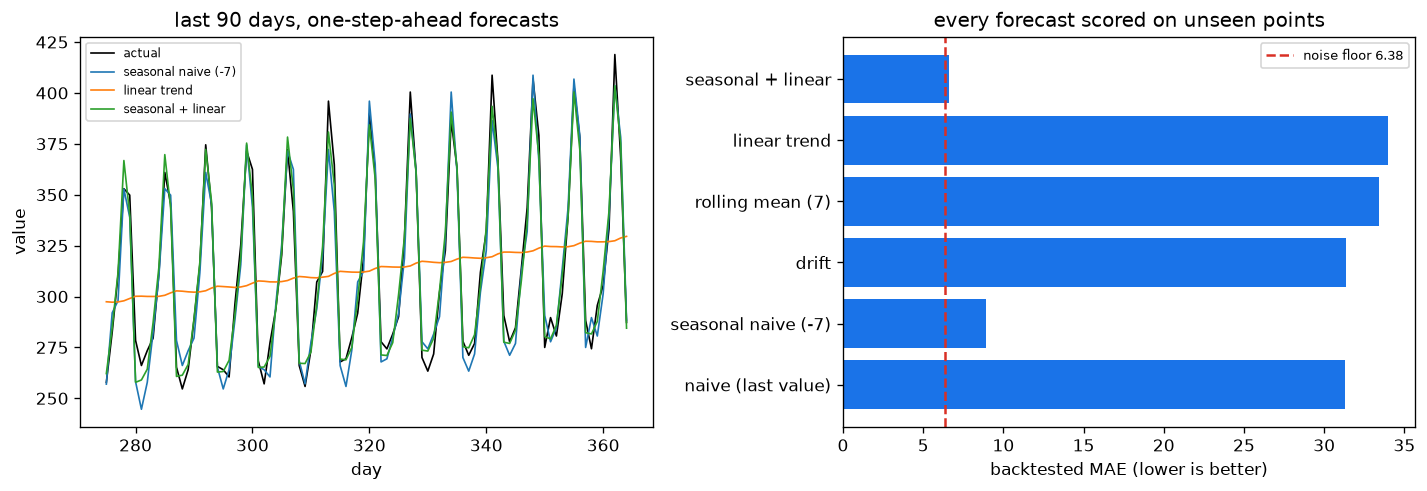
- The winner has less headroom than the table implies. The series carries N(0, 8) noise, so the best achievable one-step MAE is about 6.383. The best method reaches 6.603 — 1.03x the floor. Most of the spread in that table is between methods that are far from it, not between good ones.
- Warm-up points cannot be scored. 365 points, 305 scored forecasts: the first 60 have no history to forecast from. Two MAEs computed over different denominators are not comparable.
- A straight line cannot represent a cycle. It averages the weekly profile away and is then wrong by it every day — which is why "linear trend" scores 33.978 against seasonal-plus-linear's 6.603.
Recap
- Measured over 305 backtested one-step forecasts: seasonal + linear 6.603, seasonal naive 8.923, drift 31.363, linear trend 33.978.
- Only one method beats the seasonal-naive baseline, and it does so by 26.0%.
- Every forecast is made from data strictly before the point it predicts. Shuffling a time series before splitting lets the model see the future.
- Decomposition is the method: divide out the weekly profile, fit the trend, multiply the profile back in.
A model is reported as 79% better than the naive baseline. Why does the choice of baseline need stating?
Show answer
B — There are several naive forecasts and they differ enormously — here last-value scores 31.318 and seasonal naive 8.923, so the same model's 'improvement' changes by a factor of three depending on which is quoted
Polynomial degree rises, in-sample R^2 rises, and backtested MAE gets worse. What is happening?
Show answer
B — Extra parameters always fit the observed points better, and fitting the noise in those points makes the next point harder to predict — R^2 measures interpolation and the backtest measures extrapolation
The series has N(0, 8) noise and the best method reaches MAE 6.603 against a floor of 6.383. What follows?
Show answer
B — There is almost nothing left to win — the remaining error is irreducible noise, so effort should go elsewhere rather than into a better model
Try it yourself
Tab indents. Press Escape, then Tab, to leave the editor. Control plus Enter runs the code; Control plus Shift plus Enter submits it.
Press Run to see what your code prints.