Real-Time Demand Forecasting

Abstract

Demand arrives one period at a time, so the forecaster may only use what it has already seen. This project replays a 200-period series, refits a rolling-window linear model on the last seven lags before each new value is revealed, and scores itself against the naive “same as last period” baseline. Measured on this machine: MAE 5.202 against the baseline’s 7.726, a 32.7% improvement.

Prerequisites

Python 3.8 or above
A code editor or IDE
Basic understanding of ML and analytics
Required libraries: pandas, scikit-learn, matplotlib

Before you Start

Install Python and the required libraries:

Install dependencies

pip install pandas scikit-learn matplotlib

Getting Started

Create a Project

Create a folder named real-time-demand-forecasting.
Open the folder in your code editor or IDE.
Create a file named real_time_demand_forecasting.py.
Copy the code below into your file.

Write the Code

Real-Time Demand Forecasting

pch.viewSource

Real-Time Demand Forecasting

"""Real-time demand forecasting.

Demand arrives one period at a time. The forecaster may only use what it has
already seen, refits on a rolling window as each new point lands, and is scored
against a naive baseline that predicts "same as last period". If the model
cannot beat that baseline it is not earning its keep.
"""

import matplotlib.pyplot as plt
import numpy as np
from sklearn.linear_model import LinearRegression


class RealTimeDemandForecaster:
    """Rolling-window linear forecaster over recent lags."""

    def __init__(self, window=40, lags=7):
        self.window = window
        self.lags = lags
        self.model = LinearRegression()
        self.history = []

    def observe(self, value):
        self.history.append(float(value))

    def _design(self):
        series = np.asarray(self.history[-self.window:], dtype=float)
        rows, targets = [], []
        for index in range(self.lags, len(series)):
            rows.append(series[index - self.lags:index])
            targets.append(series[index])
        return np.asarray(rows), np.asarray(targets)

    def ready(self):
        return len(self.history) >= self.lags + 5

    def forecast(self):
        """Predict the next period from the lags seen so far."""
        if not self.ready():
            return self.history[-1] if self.history else 0.0
        rows, targets = self._design()
        self.model.fit(rows, targets)
        recent = np.asarray(self.history[-self.lags:], dtype=float)
        return float(self.model.predict(recent.reshape(1, -1))[0])


def demand_series(periods=200, seed=0):
    """Weekly seasonality, a slow trend and noise -- no leakage of the future."""
    rng = np.random.default_rng(seed)
    time = np.arange(periods)
    seasonal = 12.0 * np.sin(2 * np.pi * time / 7.0)
    trend = 0.08 * time
    noise = rng.normal(0, 4.0, periods)
    return 100.0 + seasonal + trend + noise


def replay(series, forecaster):
    """Walk the series forward, forecasting before each value is revealed."""
    model_errors, naive_errors, predictions = [], [], []
    for index, actual in enumerate(series):
        predicted = forecaster.forecast()
        naive = forecaster.history[-1] if forecaster.history else actual
        if forecaster.ready():
            model_errors.append(abs(predicted - actual))
            naive_errors.append(abs(naive - actual))
            predictions.append((index, predicted))
        forecaster.observe(actual)
    return np.asarray(model_errors), np.asarray(naive_errors), predictions


def main():
    series = demand_series()
    forecaster = RealTimeDemandForecaster()
    model_errors, naive_errors, predictions = replay(series, forecaster)

    model_mae = model_errors.mean()
    naive_mae = naive_errors.mean()
    print("Real-Time Demand Forecasting")
    print(f"  periods replayed      : {len(series)}")
    print(f"  scored forecasts      : {len(model_errors)}")
    print(f"  rolling model MAE     : {model_mae:.3f}")
    print(f"  naive (last value) MAE: {naive_mae:.3f}")
    improvement = (naive_mae - model_mae) / naive_mae
    print(f"  improvement over naive: {improvement:.1%}")
    if model_mae >= naive_mae:
        print("  the model does NOT beat the baseline on this series")

    steps, values = zip(*predictions)
    figure, axes = plt.subplots(2, 1, figsize=(9, 5), height_ratios=(2, 1))
    axes[0].plot(series, label="actual demand", linewidth=1.4)
    axes[0].plot(steps, values, label="one-step forecast", linewidth=1.2)
    axes[0].set_ylabel("units")
    axes[0].set_title("forecasting one period ahead, refitting as data arrives")
    axes[0].legend(fontsize=8)
    axes[1].plot(steps, model_errors, label=f"model (MAE {model_mae:.2f})",
                 linewidth=1.0)
    axes[1].plot(steps, naive_errors, label=f"naive (MAE {naive_mae:.2f})",
                 linewidth=1.0, alpha=0.7)
    axes[1].set_xlabel("period")
    axes[1].set_ylabel("absolute error")
    axes[1].legend(fontsize=8)
    figure.tight_layout()
    plt.savefig("real_time_demand_forecasting.png", dpi=120,
                bbox_inches="tight")
    print("saved real_time_demand_forecasting.png")


if __name__ == "__main__":
    main()

Example Usage

Run demand forecasting

python real_time_demand_forecasting.py

What it produces

Running the file exactly as it ships takes 3.7 s and prints:

python real_time_demand_forecasting.py

Real-Time Demand Forecasting
  periods replayed      : 200
  scored forecasts      : 188
  rolling model MAE     : 5.202
  naive (last value) MAE: 7.726
  improvement over naive: 32.7%
saved real_time_demand_forecasting.png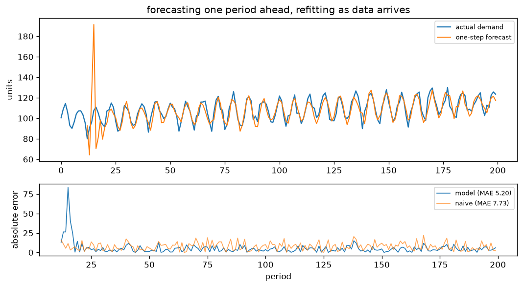

Output of real_time_demand_forecasting.py, produced by running the file. — Written by the run above. If the project stops producing it, the page's figure asset goes missing and check_docs reports it — which is the point of generating it rather than drawing it.

How it fits together

Read from the top: this is what runs when you execute the file, and which function calls which. It is generated from the code, so it cannot drift from it.

diagram Diagram mermaid

  flowchart TD
  RUN(["python real_time_demand_forecasting.py"])
  RealTimeDemandForecaster["RealTimeDemandForecaster
class"]
  demand_series("demand_series")
  replay("replay")
  main("main")
  RUN --> main
  main --> RealTimeDemandForecaster
  main --> demand_series
  main --> replay

Explanation