Activation Functions (ReLU, Sigmoid, Softmax)

Every layer you have built so far ends with activation="relu" or "softmax". This page is about that small non-linear function, and it makes three claims with numbers attached: without it a deep network is algebraically one layer, the choice of activation decides whether a deep network trains at all, and the usual advice (“always ReLU”) does not survive contact with the measurement.

What you’ll learn

• Why stacking linear layers collapses into a single one — proved in two lines and verified to $8.88 \times 10^{-16}$.
• The exact derivative of each activation, and why the sigmoid’s ceiling of 0.25 is the whole vanishing-gradient story.
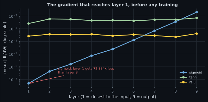
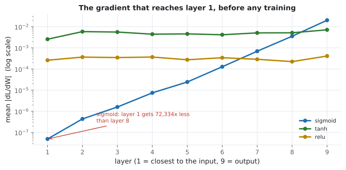
• The gradient that actually reaches layer 1 of an 8-layer network: 72,334× smaller with sigmoid than with tanh or ReLU, measured before a single update.
• Softmax and cross-entropy derived together, ending in the gradient $\hat{\mathbf{p}} - \mathbf{y}$ — checked against a numeric gradient to $10^{-10}$.
• How to pick the output layer from the shape of the problem, not from habit.
• Two measured results that contradict the folklore: tanh does not degrade at depth 8 (0.8782 against ReLU’s 0.8502), and dead ReLU units stayed under 4% at every learning rate tested.

Why a network needs a non-linearity at all

Take two Dense layers with no activation. The first computes $\mathbf{h} = \mathbf{x}\mathbf{W}_1 + \mathbf{b}_1$, the second $\mathbf{y} = \mathbf{h}\mathbf{W}_2 + \mathbf{b}_2$. Substitute:

$$\mathbf{y} = (\mathbf{x}\mathbf{W}_1 + \mathbf{b}_1)\mathbf{W}_2 + \mathbf{b}_2 = \mathbf{x}\underbrace{(\mathbf{W}_1\mathbf{W}_2)}_{\mathbf{W}'} + \underbrace{(\mathbf{b}_1\mathbf{W}_2 + \mathbf{b}_2)}_{\mathbf{b}'}$$

The composition is $\mathbf{x}\mathbf{W}' + \mathbf{b}'$ — a single linear layer with $\mathbf{W}' = \mathbf{W}_1\mathbf{W}_2$ and $\mathbf{b}' = \mathbf{b}_1\mathbf{W}_2 + \mathbf{b}_2$. This is not an approximation or a rule of thumb; it is matrix multiplication being associative. Stack a hundred linear layers and the same substitution collapses all of them.

Run it and the two agree to floating-point noise:

linear_collapse.py

import numpy as np
 
rng = np.random.default_rng(0)
W1, b1 = rng.normal(size=(3, 4)), rng.normal(size=4)
W2, b2 = rng.normal(size=(4, 2)), rng.normal(size=2)
x = rng.normal(size=(5, 3))
 
stacked = (x @ W1 + b1) @ W2 + b2            # two layers
W_eq, b_eq = W1 @ W2, b1 @ W2 + b2           # one equivalent layer
collapsed = x @ W_eq + b_eq
 
print("max difference:", f"{np.abs(stacked - collapsed).max():.2e}")
# max difference: 8.88e-16
print("equivalent layer:", W_eq.shape, b_eq.shape)
# equivalent layer: (3, 2) (2,)

What that costs on real data. Three-class spiral, 450 training points, two hidden layers of 32 units, 120 epochs, identical seeds — the only difference is whether the hidden layers have an activation:

Model	Parameters	Test accuracy
2 hidden layers, no activation	1,251	0.7000
2 hidden layers, ReLU	1,251	0.9933
a single Dense(3) layer	9	0.6667

The linear stack carries 139× more parameters than the single layer and buys 0.0333 accuracy for them — noise from a different optimisation path, not capacity. Adding relu to the same 1,251 parameters buys 0.2933. The parameters were never the constraint; the linearity was.

The four activations, and what their derivatives cost

$$\sigma(z) = \frac{1}{1 + e^{-z}} \qquad \tanh(z) = \frac{e^{z} - e^{-z}}{e^{z} + e^{-z}} \qquad \mathrm{ReLU}(z) = \max(0, z)$$

Backpropagation multiplies one derivative per layer, so the derivative — not the activation — decides what happens at depth:

$$\sigma'(z) = \sigma(z)\bigl(1 - \sigma(z)\bigr) \qquad \tanh'(z) = 1 - \tanh^{2}(z) \qquad \mathrm{ReLU}'(z) = \begin{cases} 1 & z > 0 \\ 0 & z < 0 \end{cases}$$

$\sigma(z)(1-\sigma(z))$ is a product of two numbers that sum to 1, so it is largest when both are $\tfrac{1}{2}$:

$$\max_z \sigma'(z) = \tfrac{1}{2} \cdot \tfrac{1}{2} = 0.25$$

figure The activation on the left; the number backpropagation actually multiplies by on the right matplotlib

Leaky ReLU is drawn dashed because it is identical to ReLU except for a 0.01 slope on the negative side. The right panel is the one that matters: tanh's derivative reaches 1.0 at the origin, ReLU's is exactly 1.0 for every positive input, and sigmoid's can never exceed 0.25 anywhere.

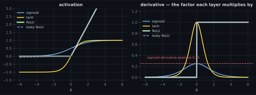
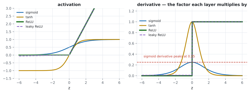
That ceiling compounds. A gradient crossing $k$ sigmoid layers is multiplied by at most $0.25^{k}$:

Layers crossed	Best case for sigmoid, $0.25^{k}$	ReLU on active units, $1^{k}$
1	0.25	1.0
2	0.0625	1.0
4	$3.906 \times 10^{-3}$	1.0
8	$1.526 \times 10^{-5}$	1.0
16	$2.328 \times 10^{-10}$	1.0

And that is the best case, at $z = 0$; anywhere else the factor is smaller.

The gradient that actually reaches layer 1

The table above is arithmetic. This is a measurement: an 8-hidden-layer network on MNIST, one batch of 256, mean $\lvert \partial L / \partial \mathbf{W} \rvert$ per layer, before any training — so nothing here is the optimiser’s fault.

figure Nine layers, three activations, one batch matplotlib

Sigmoid's first layer receives a gradient of 4.89e-08 while its last receives 2.02e-02 — a factor of 72,334. The tanh and ReLU curves are flat, which is the entire practical argument for both: the update reaching layer 1 is the same order of magnitude as the update reaching layer 9.

Activation	layer 1	layer 8	ratio (layer 1 ÷ layer 8)
sigmoid	$4.89 \times 10^{-8}$	$3.54 \times 10^{-3}$	$1.38 \times 10^{-5}$
tanh	$2.56 \times 10^{-3}$	$5.14 \times 10^{-3}$	0.498
relu	$2.59 \times 10^{-4}$	$2.23 \times 10^{-4}$	1.16

Note what the sigmoid network is not doing: it is not saturated. Measured on 1,000 test images at initialisation, 0.0000 of its activations exceed 0.99 in absolute value, at layer 1 and at layer 8. The gradient is tiny because of the 0.25 ceiling multiplying eight times, not because any unit is stuck. Saturation makes it worse later; the arithmetic is already fatal at initialisation.

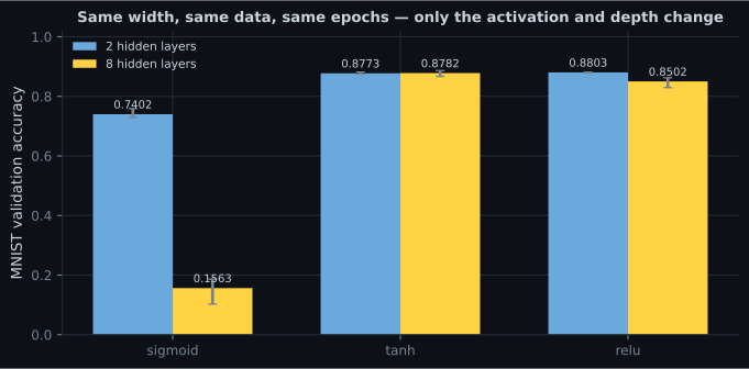
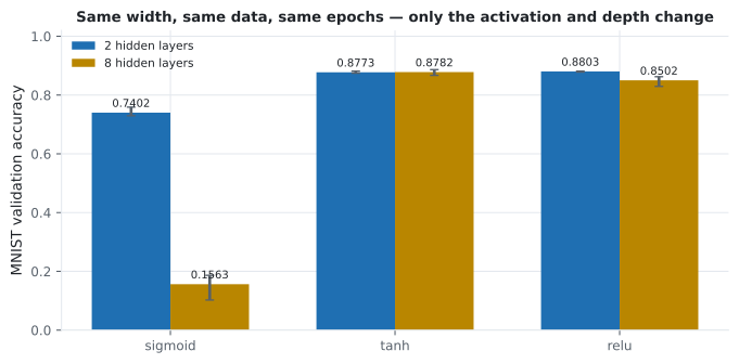
Does it change the accuracy? Measured

Same width, same data, same epochs, three seeds each — only the activation and the depth change:

figure MNIST validation accuracy, 8,000 rows, 4 epochs, 3 seeds (bars are the mean, whiskers the range) matplotlib

Sigmoid at depth 8 collapses to 0.1563 — barely above the 0.10 you get by always guessing one class. tanh is unmoved by the extra six layers. ReLU loses 0.03 at depth 8 in this budget, which is a real result and not the one the folklore predicts.

Activation	2 hidden layers	8 hidden layers
sigmoid	0.7402 (0.7295–0.7590)	0.1563 (0.1025–0.1865)
tanh	0.8773 (0.8745–0.8815)	0.8782 (0.8670–0.8865)
relu	0.8803 (0.8785–0.8815)	0.8502 (0.8295–0.8625)

Three readings, and the third is the uncomfortable one:

Depth is what makes the activation matter. At two layers, sigmoid is 0.14 behind and everything else is within noise. At eight, sigmoid stops learning entirely.

tanh did not degrade. 0.8782 at depth 8 against 0.8773 at depth 2 — the extra six layers cost nothing measurable. Its derivative reaches 1.0 at the origin and its outputs are zero-centred, which is exactly what the gradient figure shows.

ReLU lost 0.0301 going deep, and lost to tanh at depth 8. “Always use ReLU” is folklore at this scale. ReLU wins on cost (a comparison and a copy, no exponential) and it wins at the widths and epoch budgets where modern networks live, but on this measurement it is second. Report what you measure.

Softmax and cross-entropy, derived together

Softmax turns $K$ real-valued logits into a distribution:

$$\mathrm{softmax}(\mathbf{z})_i = \frac{e^{z_i}}{\sum_{j=1}^{K} e^{z_j}}$$

Every output is positive and they sum to 1 by construction. Paired with it, categorical cross-entropy scores the prediction against a one-hot target $\mathbf{y}$:

$$L = -\sum_{i=1}^{K} y_i \log \hat{p}_i = -\log \hat{p}_c$$

for true class $c$ — only one term survives, because $\mathbf{y}$ is one-hot.

Worked by hand

Logits $\mathbf{z} = [2.0,\ 1.0,\ 0.1]$:

$$e^{\mathbf{z}} = [7.389056,\ 2.718282,\ 1.105171], \qquad \textstyle\sum_j e^{z_j} = 11.212509$$ $$\hat{\mathbf{p}} = [0.659001,\ 0.242433,\ 0.098566]$$

The loss depends entirely on which class is true:

True class	$\hat{p}_c$	$L = -\log \hat{p}_c$
0	0.659001	0.417030
1	0.242433	1.417030
2	0.098566	2.317030

Note the spacing: the differences are exactly $\log$ ratios of the probabilities, so being confidently wrong is punished without bound while being confidently right approaches zero loss but never reaches it.

The gradient is a subtraction

Differentiate the pair together and everything cancels:

$$\frac{\partial L}{\partial z_i} = \hat{p}_i - y_i$$

For our example with true class 0, $\hat{\mathbf{p}} - \mathbf{y} = [-0.340999,\ 0.242433,\ 0.098566]$. A central-difference gradient of the same loss gives the same three numbers to $1.05 \times 10^{-10}$. Two properties fall out for free: the components sum to exactly zero (softmax outputs are constrained to sum to 1, so pushing one logit up must push others down), and no derivative of the activation appears anywhere — which is why this pairing trains when sigmoid-plus-squared-error does not.

Never apply softmax twice

loss="categorical_crossentropy" expects probabilities; from_logits=True expects raw logits and applies the softmax internally, in a numerically stable way. Doing both — softmax in the last layer and from_logits=True — silently trains a model on softmax-of-softmax, which flattens the distribution and quietly costs accuracy with no error message.

Why the implementation subtracts the max

$e^{1000}$ overflows to inf in float64, and inf / inf is nan. Since softmax is unchanged by shifting every logit by a constant, subtract the largest one first:

$$\mathrm{softmax}(\mathbf{z})_i = \frac{e^{z_i - \max_j z_j}}{\sum_j e^{z_j - \max_j z_j}}$$

stable_softmax.py

import numpy as np
 
def softmax(v):
    shifted = v - v.max()          # the whole trick: largest exponent becomes 0
    exponent = np.exp(shifted)
    return exponent / exponent.sum()
 
large = np.array([1000.0, 999.0, 998.0])
print(softmax(large))                                  # [0.665241 0.244728 0.090031]
print(np.exp(large) / np.exp(large).sum())             # [nan nan nan]

Temperature: the same logits, a different distribution

Dividing the logits by a temperature $T$ before the softmax rescales confidence without changing the ranking. It is how text generation trades safety for surprise, and it appears again in Phase 06:

$T$	probabilities	top probability
0.25	[0.9815, 0.0180, 0.0005]	0.9815
0.50	[0.8638, 0.1169, 0.0193]	0.8638
1.00	[0.6590, 0.2424, 0.0986]	0.6590
2.00	[0.5017, 0.3043, 0.1940]	0.5017
10.00	[0.3661, 0.3312, 0.3027]	0.3661

As $T \to 0$ softmax becomes $\arg\max$; as $T \to \infty$ it becomes uniform.

Choosing the output layer

The output activation is not a preference — it is determined by what a prediction is for your problem:

diagram Diagram mermaid

  flowchart TD
  A["What is one prediction?"] --> B{"A real number"}
  A --> C{"One of two classes"}
  A --> D{"One of K classes,
exactly one true"}
  A --> E{"Any subset of K labels"}
  B --> B1["No activation.
loss = mse or mae"]
  B --> B2{"Bounded target?"}
  B2 -->|"must be positive"| B3["relu or softplus"]
  B2 -->|"known range"| B4["sigmoid or tanh,
and scale the labels to match"]
  C --> C1["Dense(1, activation='sigmoid')
loss = binary_crossentropy"]
  D --> D1["Dense(K, activation='softmax')
loss = categorical_crossentropy"]
  E --> E1["Dense(K, activation='sigmoid')
loss = binary_crossentropy
K independent yes/no questions"]
  E1 --> E2["softmax here is a BUG:
it forces the labels to sum to 1"]

The bottom-right branch is the one that bites. Tagging an email as both “spam” and “urgent” needs two independent sigmoids; softmax would force $P(\text{spam}) + P(\text{urgent}) = 1$, encoding “it cannot be both” into the architecture:

multilabel_output.py

from tensorflow import keras
 
model = keras.Sequential([
    keras.layers.Input((10,)),
    keras.layers.Dense(16, activation="relu"),
    keras.layers.Dense(2, activation="sigmoid"),      # 2 independent labels
])
model.compile(loss="binary_crossentropy", optimizer="rmsprop", metrics=["accuracy"])

For hidden layers the default is ReLU, with tanh worth trying whenever the network is deep and unnormalised — the measurement above is a direct argument for testing both rather than assuming.

See it move

The first sketch shows the shapes; the second shows the compounding that the shapes imply. Drag the depth slider and watch a gradient of 1.0 shrink as it crosses layers.

sketch Activation functions reshape the signal p5.js Pause Restart

ReLU clips negatives to zero, sigmoid squashes to 0..1, tanh squashes to -1..1. A sweeping probe shows what each function outputs for the same input, in real time.

sketch One derivative per layer, multiplied p5.js Pause Restart

A gradient of 1.0 enters at the output and crosses layer after layer, multiplied by each activation's derivative. The sigmoid chain collapses within a few layers; tanh and ReLU arrive intact. Drag to change the depth.

At depth 8 the sigmoid chain is down to $1.53 \times 10^{-5}$ of its original size while ReLU is unchanged — which is the same conclusion the measured figure reached by a completely different route, from real gradients in a real network.

Pitfalls

Softmax on a multilabel problem. Forces the predicted labels to sum to 1. Use one sigmoid per label. This is an architecture bug, not a tuning issue — no amount of training fixes it.

Applying softmax twice. A softmax output layer plus from_logits=True is softmax-of-softmax. It trains, it never errors, and it silently flattens every prediction.

Reading “dead ReLU” as a routine emergency. Measured on four learning rates, after 4 epochs on 8,000 MNIST rows with a 4×64 network:

Learning rate	Dead units	Test accuracy
0.001	3 / 256 (1.17%)	0.1210
0.01	6 / 256 (2.34%)	0.4500
0.1	9 / 256 (3.52%)	0.8640
0.5	5 / 256 (1.95%)	0.8690

Dead units never exceeded 3.52%, and they did not rise monotonically with the learning rate. What actually separated these runs was training progress: at lr 0.001 the network had barely started (0.1210). Dead ReLUs are real and worth knowing about; on this evidence they were not what limited any of these models. Measure before reaching for leaky ReLU.

Expecting sigmoid hidden layers to work if you just train longer. At depth 8 the first layer receives $4.89 \times 10^{-8}$ of gradient at initialisation. Longer training multiplies a number that is already negligible.

Assuming ReLU is always the best hidden activation. On the measurement on this page, tanh beat it at depth 8 (0.8782 against 0.8502). Try both; it is two characters of code.

Forgetting to scale labels when the output is bounded. A sigmoid output cannot emit 350,000. If the output activation bounds the range, the labels have to live in that range too.

Recap

• Two linear layers are one linear layer: $\mathbf{W}' = \mathbf{W}_1\mathbf{W}_2$, verified to $8.88\times10^{-16}$. On the spiral, adding relu to the same 1,251 parameters moved accuracy from 0.7000 to 0.9933.
• $\sigma'(z) \le 0.25$ everywhere, so eight sigmoid layers multiply a gradient by at most $1.526\times10^{-5}$. Measured in a real 8-layer network, layer 1 received 72,334× less gradient than layer 8.
• Accuracy follows: sigmoid 0.7402 → 0.1563 from depth 2 to 8, tanh 0.8773 → 0.8782, ReLU 0.8803 → 0.8502.
• Softmax with cross-entropy has gradient $\hat{\mathbf{p}} - \mathbf{y}$, which contains no activation derivative — checked against a numeric gradient to $1.05\times10^{-10}$.
• Subtract the max before exponentiating, or large logits produce nan.
• The output layer follows from the problem shape: none for regression, one sigmoid for binary, softmax for single-label multiclass, K sigmoids for multilabel.
• Dead ReLU units stayed under 4% at every learning rate tested here — check yours rather than assuming.

pch.quizTag pch.quizDefaultTitle

1. You stack five Dense layers with no activation function. What have you built?

   A A deep network that needs more epochs to train B Exactly one linear layer — the five weight matrices multiply into a single W' and the biases into a single b', verified here to 8.88e-16 C A network that will overfit because of its depth D A network equivalent to one layer only if all the layers are the same width
   pch.quizShowAnswer

   B — Exactly one linear layer — the five weight matrices multiply into a single W' and the biases into a single b', verified here to 8.88e-16 — Matrix multiplication is associative, so (xW1+b1)W2+b2 = xW1W2 + (b1W2+b2). The collapse holds for any widths and any depth. The measurement on this page: 1,251 parameters with no activation scored 0.7000 on the spiral, against 0.9933 for the same 1,251 with relu.

2. Why does a sigmoid network with 8 hidden layers fail to train, on the evidence here?

   A Its units are saturated at initialisation B Because the sigmoid derivative can never exceed 0.25, so eight layers multiply the gradient by at most 1.5e-05 — measured, layer 1 received 72,334x less gradient than layer 8, while 0.0000 of its activations were above 0.99 C Sigmoid outputs are not zero-centred, which is the whole problem D The learning rate is always too low for sigmoid
   pch.quizShowAnswer

   B — Because the sigmoid derivative can never exceed 0.25, so eight layers multiply the gradient by at most 1.5e-05 — measured, layer 1 received 72,334x less gradient than layer 8, while 0.0000 of its activations were above 0.99 — Saturation was measured at exactly 0.0000 of activations above 0.99 at initialisation — the units are not stuck. The 0.25 ceiling compounding across eight layers is enough on its own, which is why the failure is visible before the first update.

3. Softmax paired with categorical cross-entropy has gradient dL/dz = p - y. Why does that matter?

   A It makes the loss smaller B No activation derivative appears in it, so nothing shrinks the signal at the output layer, and the components sum to exactly zero C It means you can skip the softmax at inference D It only holds when there are exactly two classes
   pch.quizShowAnswer

   B — No activation derivative appears in it, so nothing shrinks the signal at the output layer, and the components sum to exactly zero — The activation derivative cancels against the loss derivative. Contrast sigmoid-plus-squared-error, where a sigma'(z) factor of at most 0.25 multiplies every output gradient. The zero sum follows from softmax outputs being constrained to sum to 1.

4. An email can be both 'spam' and 'urgent'. What output layer do you use for two such labels?

   A Dense(2, activation='softmax') with categorical_crossentropy B Dense(2, activation='sigmoid') with binary_crossentropy — two independent yes/no questions whose probabilities need not sum to 1 C Dense(1, activation='sigmoid') and threshold it twice D Dense(2) with no activation and mse
   pch.quizShowAnswer

   B — Dense(2, activation='sigmoid') with binary_crossentropy — two independent yes/no questions whose probabilities need not sum to 1 — Softmax would force P(spam) + P(urgent) = 1, encoding 'it cannot be both' into the architecture. Independent sigmoids let both be 0.9 at once.

5. Your softmax returns nan for a batch of large logits. What is the fix?

   A Lower the learning rate B Subtract the maximum logit before exponentiating — softmax is invariant to that shift, and it turns exp(1000) into exp(0) C Clip the logits to [-1, 1] D Switch to float64
   pch.quizShowAnswer

   B — Subtract the maximum logit before exponentiating — softmax is invariant to that shift, and it turns exp(1000) into exp(0) — exp(1000) overflows to inf and inf/inf is nan. Shifting by the max leaves the result unchanged mathematically: the same logits give [0.665241, 0.244728, 0.090031] instead of nan. Clipping would change the distribution; float64 only moves the overflow point.

Next

You now know what each activation does to the signal and to the gradient. Continue to Building Neural Networks with Keras (Sequential and Functional API) to see how these layers get assembled into a model — and then to How Neural Networks Learn, where the gradients measured here are actually used to update weights.

🧪 Try It Yourself

Exercise 1 – Every activation and its derivative

pch.exerciseTag pch.exerciseTitle

Exercise 2 – Collapse a linear stack yourself

pch.exerciseTag pch.exerciseTitle

Exercise 3 – A softmax that survives large logits

pch.exerciseTag pch.exerciseTitle

Exercise 4 – Check the softmax + cross-entropy gradient

pch.exerciseTag pch.exerciseTitle

Exercise 5 – Temperature reshapes the same logits

pch.exerciseTag pch.exerciseTitle

Exercise 6 – Count the silent units

pch.exerciseTag pch.exerciseTitle