Diffusion Models (Introduction)

A diffusion model is trained to do one narrow thing: given a noisy image and the amount of noise in it, predict the noise. That makes it the easiest generative family to verify, because the forward process — the corruption the model learns to undo — has a closed form. Every claim about it can be checked with arithmetic instead of trained.

$$x_t = \sqrt{\bar\alpha_t}\, x_0 + \sqrt{1 - \bar\alpha_t}\, \epsilon, \qquad \epsilon \sim \mathcal{N}(0, I), \qquad \bar\alpha_t = \prod_{s \le t}(1 - \beta_s)$$

One equation gets you to any timestep in a single step — no simulation, no loop. The model’s whole job is to invert it.

The first version of this page produced blobs, and it had two plausible explanations. Both were tested. One was wrong.

Run	Training loss	Signal weight at last step	Mean ink	Classes	KL from uniform
Dense, original schedule	0.8804	0.3636	0.4737	2	12.9494
Dense, terminal-SNR fixed	0.8738	0.0466	0.4780	2	14.4285
Convolutional, same fix	0.0314	0.0466	0.0503	7	2.5506
Real digits	—	—	0.1192	10	0.0360

The schedule fix — the obvious suspect, and a real published problem — changed nothing. The architecture change was worth a 28× reduction in training loss.

What you’ll learn

• The forward process in closed form, and how to read a noise schedule from its numbers.
• The terminal SNR problem: why a schedule that never fully destroys the image is broken, and why fixing it here still did not fix the samples.
• Why a dense network is the wrong shape for denoising, measured.
• Why more reverse steps made coverage worse — 0.2495 at 20 steps against 2.5506 at 200 — while costing 11× more time.

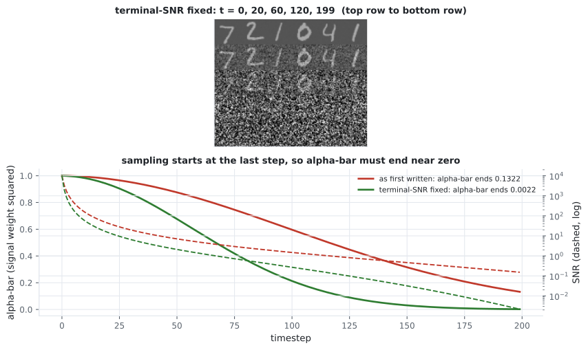
The forward process

The schedule is a design choice, and every property of it is arithmetic:

figure 200 steps, linear beta matplotlib

The bottom panel is the whole design decision. Sampling starts at the LAST timestep from pure Gaussian noise, so alpha-bar has to end near zero or the model is asked to denoise something it never saw in training. The original schedule ends at 0.1322 — the image still contributes 0.3636 of the signal — while the fixed one ends at 0.0022.

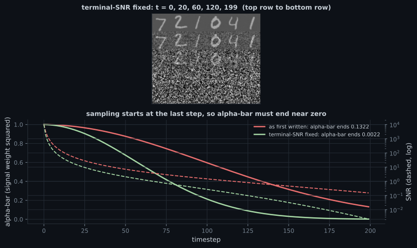
t	β	$\bar\alpha_t$	Signal weight	Noise weight	SNR
0	0.00010	0.99990	0.9999	0.0100	9999.0000
20	0.00210	0.97715	0.9885	0.1512	42.7609
60	0.00610	0.82738	0.9096	0.4155	4.7931
120	0.01210	0.47659	0.6904	0.7235	0.9105
199	0.02000	0.13218	0.3636	0.9316	0.1523

That last row is a genuine defect, known in the literature as the terminal signal-to-noise problem. At the final timestep the image is still a third of the signal, so the training distribution at $t = 199$ and the sampling distribution (pure noise) do not match. Raising $\beta_{\max}$ from 0.02 to 0.06 fixes it: the final signal weight drops to 0.0466 and SNR to 0.0022.

The fix that did not work

Training: predict the noise, not the image

timesteps = rng.integers(0, STEPS, len(clean))
noisy, noise = add_noise(clean, timesteps)          # the closed form above
 
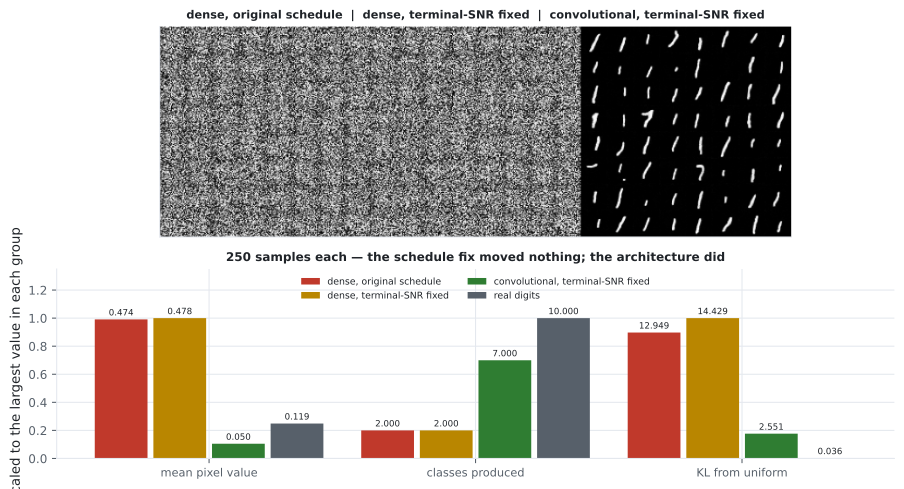
model.fit([noisy, embed(timesteps)], noise, ...)    # target is the NOISE

With the schedule corrected and everything else unchanged, the samples did not improve — they got marginally worse, KL 12.9494 → 14.4285, both at 2 of 10 classes. The tell was in a column that is easy to skip:

Mean ink. Real MNIST digits average 0.1192 per pixel. The dense model’s samples averaged 0.4737 and 0.4780 — four times as much. That is not a subtly wrong distribution, it is a model smearing brightness across the whole canvas, which is what a network with no spatial structure does when asked to remove spatially structured noise.

figure 250 samples per run, 200 reverse steps, same judge matplotlib

Two hypotheses, one figure. Rows 1 and 2 differ only in the noise schedule and are indistinguishable in outcome — the terminal-SNR fix was not the problem. Row 3 changes the denoiser from three dense layers to a small U-Net with the same schedule, and mean ink falls from 0.4780 to 0.0503 against real data's 0.1192, with classes produced rising from 2 to 7.

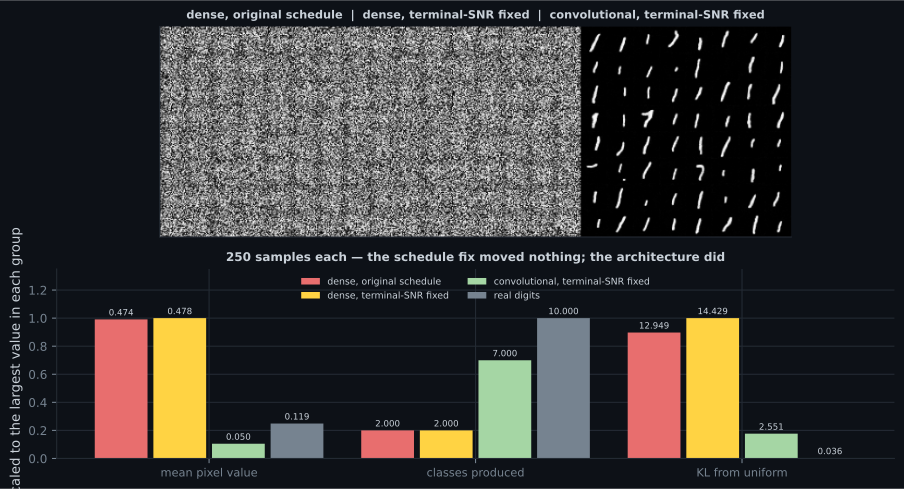
The convolutional denoiser is a small U-Net: two downsampling stages, a bottleneck, two upsampling stages with skip connections, and the timestep embedding added as a per-channel bias at each scale.

Why a convolution and not a dense layer

first = keras.layers.Conv2D(32, 3, padding="same", activation="relu")(x)
first = add_time(first, 32)                      # timestep as a channel bias
down = keras.layers.MaxPooling2D()(first)
...
up = keras.layers.Concatenate()([up, first])     # skip: fine detail comes back

Denoising is a local operation — each pixel’s correct value depends mostly on its neighbours. A dense layer must learn that neighbourhood relationship from scratch out of a flat vector of 784 inputs; a convolution is handed it. With fewer parameters (160,225 against 538,128) the U-Net reached a training loss of 0.0314 against 0.8738.

It cost 2,723 seconds against 69, which is the honest other side of that trade.

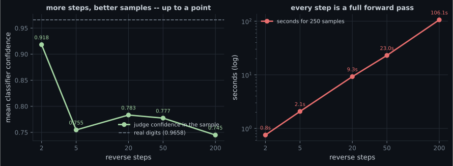
More steps made it worse

The reverse process runs the model once per step. Standard advice is that more steps give better samples, and the cost is linear. The cost part is true:

figure The convolutional model, terminal-SNR fixed matplotlib

Cost is linear in steps because every step is a full forward pass over the whole batch — 0.8s at 2 steps, 106.1s at 200. Confidence is highest at 2 steps (0.9183), which is a warning rather than a result: a confident classification of a bright blob is still a bright blob, as the coverage table below shows.

Reverse steps	Seconds	Classes	KL from uniform	Mean ink	Judge confidence
2	0.8	3	11.2875	0.4939	0.9183
5	2.1	10	0.3567	0.1076	0.7547
20	9.3	10	0.2495	0.0812	0.7833
50	23.0	9	0.5740	0.0686	0.7774
200	106.1	7	2.5506	0.0503	0.7449

Coverage peaks at 20 steps and then degrades. Going from 20 to 200 steps costs 11× the time and loses three classes.

Two things are happening, and the mean-ink column separates them:

1. Two steps is genuinely too few. Ink 0.4939, three classes — the sampler has not had time to resolve anything, and the judge’s high confidence (0.9183) is confidence about blobs.
2. Two hundred steps over-denoises. Ink falls monotonically with step count — 0.1076, 0.0812, 0.0686, 0.0503 — dropping below real data’s 0.1192. Each step re-estimates the clean image and clips it to a valid range, so many small steps accumulate a bias towards thin, faint strokes, and the variety of digits collapses with it.

That second effect is specific to this sampler (predict $x_0$, re-noise with fresh noise) and this model. The general lesson is not “use 20 steps” — it is that step count is a hyperparameter with a measurable optimum, not a dial where more is always better. Nothing on the sample grid announces that 200 steps was worse than 20.

diagram Diagram mermaid

  flowchart LR
  X0["clean image"] -->|"forward: closed form,
one step to any t"| XT["x_t"]
  XT -->|"model predicts the noise"| E["epsilon-hat"]
  E --> X0H["implied clean image"]
  X0H -->|"re-noise to t-1"| XT
  XT -->|"t = 0"| OUT["sample"]
  E -.->|"dense: loss 0.8738"| BAD["ink 0.4780, 2 classes"]
  E -.->|"convolutional: loss 0.0314"| GOOD["ink 0.0503, 7 classes"]

sketch Design a noise schedule p5.js Pause Restart

Drag the slider to change beta_max. The curve is alpha-bar over 200 steps, and the readout is the value that decides whether sampling starts in-distribution.

What the model actually predicts

figure The convolutional denoiser at three noise levels matplotlib

The third column is the network's actual output — the noise, not the image. The fourth is what that implies about the clean image, obtained by rearranging the forward equation. At the highest noise level the predicted noise is visibly smoother than the true noise: the model cannot recover the specific noise sample, only its best estimate, and that gap is exactly the irreducible part of the loss.

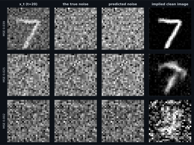
Predicting the noise rather than the image looks arbitrary and is not. The two are related by a rearrangement, so they carry the same information — but the noise target has constant scale across all timesteps, while the clean-image target does not. That keeps the loss comparable at every noise level, which is what lets one network handle the whole schedule.

sketch The measured table, ranked p5.js Pause Restart

Click a column to rank every row by it. The bars are that column's values and the highest and lowest are computed from the numbers, not written in.

Pitfalls

• A schedule that does not end near zero. The original ended with the image at 0.3636 of the signal, so sampling started off-distribution. Check $\bar\alpha_T$ before anything else.
• Assuming the schedule is the problem. Fixing it here moved KL from 12.9494 to 14.4285 — the wrong direction. The architecture was the bottleneck.
• Using a dense network as the denoiser. With 3.4× more parameters it reached a 28× higher training loss.
• Believing more reverse steps are always better. Coverage peaked at 20 steps (KL 0.2495) and degraded to 2.5506 at 200, for 11× the cost.
• Reading classifier confidence as sample quality. It was highest at 2 steps (0.9183), the worst setting on every other measure.
• Timing the sampler on its first call. The first version of this module reported 2 steps as the slowest setting (56.3s against 1.0s for 5 steps) because model training happened inside the timed block.
• Comparing these numbers with published diffusion results. This is MNIST at 28×28 with a 160k-parameter U-Net on a CPU.

Recap

• The forward process has a closed form, so the schedule can be verified with arithmetic instead of experiments.
• Terminal SNR matters — a schedule ending at signal weight 0.3636 is broken — but fixing it did not fix these samples.
• The denoiser’s architecture did: a 160,225-parameter U-Net reached training loss 0.0314 where a 538,128-parameter dense network reached 0.8738.
• Mean pixel value was the diagnostic that identified the cause: 0.4780 for dense samples against 0.1192 for real digits.
• Sampling cost is linear in steps (0.8s to 106.1s), and coverage peaked at 20 steps rather than at the maximum.
• The model predicts the noise because that target has constant scale across timesteps.

Next

Diffusion, GANs and VAEs are all judged by the same three measurements, and each of those can be gamed — including by a model that copies its training data: Evaluating Generative Models.

pch.quizTag pch.quizDefaultTitle

1. Why must a noise schedule's alpha-bar end near zero?

   A To keep the training loss small B Because sampling starts at the last timestep from pure Gaussian noise — if the image still contributes signal there, the sampler begins from a distribution the model never saw in training C Because beta must sum to 1 D To make the forward process reversible
   pch.quizShowAnswer

   B — Because sampling starts at the last timestep from pure Gaussian noise — if the image still contributes signal there, the sampler begins from a distribution the model never saw in training — The original schedule here ended with the image at 0.3636 of the signal. That is a real defect, even though fixing it did not fix these particular samples.

2. Correcting the terminal SNR moved coverage KL from 12.9494 to 14.4285. What was the right conclusion?

   A The correction was implemented wrongly B The hypothesis was wrong — the schedule was not what was limiting the samples, so the next suspect had to be tested rather than the fix being credited C Coverage KL is not a valid metric D The model needed more training epochs
   pch.quizShowAnswer

   B — The hypothesis was wrong — the schedule was not what was limiting the samples, so the next suspect had to be tested rather than the fix being credited — A fix that does not move the outcome has not been shown to help. The architecture change moved training loss from 0.8738 to 0.0314.

3. The convolutional denoiser had 160,225 parameters against the dense network's 538,128, yet reached a far lower loss. Why?

   A It trained for more epochs B Denoising is a local operation, and a convolution is given the neighbourhood structure that a dense layer has to learn from a flat 784-value vector C It used a better optimiser D Skip connections add parameters that are not counted
   pch.quizShowAnswer

   B — Denoising is a local operation, and a convolution is given the neighbourhood structure that a dense layer has to learn from a flat 784-value vector — Parameter count is not capability. Matching the architecture to the structure of the problem beat having three times as many weights.

4. Coverage KL was 0.2495 at 20 reverse steps and 2.5506 at 200, while sampling time rose from 9.3s to 106.1s. What does this show?

   A The 200-step run was not given enough time B Step count has a measurable optimum rather than being a more-is-better dial; here the extra steps over-denoised, with mean ink falling to 0.0503 against real data's 0.1192 C The judge classifier degrades on longer runs D Coverage KL is unreliable above 50 steps
   pch.quizShowAnswer

   B — Step count has a measurable optimum rather than being a more-is-better dial; here the extra steps over-denoised, with mean ink falling to 0.0503 against real data's 0.1192 — Each step re-estimates and clips the clean image, so many steps accumulate a bias towards faint, thin strokes — and no sample grid would announce that.

5. Why is the training target the noise rather than the clean image?

   A The noise is easier to compute B The two are equivalent by rearrangement, but the noise target has constant scale at every timestep, which keeps the loss comparable across the whole schedule C Predicting the image would require a discriminator D Because the clean image is unknown during training
   pch.quizShowAnswer

   B — The two are equivalent by rearrangement, but the noise target has constant scale at every timestep, which keeps the loss comparable across the whole schedule — One network has to serve every noise level, so a target whose scale does not change with t is what makes a single loss meaningful.

🧪 Try It Yourself

pch.exerciseTag pch.exerciseTitle

pch.exerciseTag pch.exerciseTitle

pch.exerciseTag pch.exerciseTitle

pch.exerciseTag pch.exerciseTitle

pch.exerciseTag pch.exerciseTitle

pch.exerciseTag pch.exerciseTitle