
Hyperparameter Tuning with GridSearchCV
What you’ll learn
Section titled “What you’ll learn”- parameters against hyperparameters, and why only one kind can be learned by fitting
- the fit-count formula, and why a grid becomes impossible faster than people expect
- reading
cv_results_— the winner is the least interesting row in it - tuning preprocessing and model together through the double-underscore path
- the edge-of-grid check, which is the most common way a search quietly under-delivers
- nested cross-validation, and the 0.4-point optimism it exposes
Intuition
Section titled “Intuition”A model has two kinds of number attached to it.
Parameters are learned by fitting: the coefficients of a linear model, the split thresholds of a tree. You never set them.
Hyperparameters are set before fitting and control how the fitting happens: C, gamma,
max_depth, n_estimators, alpha. Nothing in the training data tells you their values, because
they govern the process that reads the training data.
So they must be chosen by search. Try a combination, cross-validate it, keep the best. Grid search is the exhaustive version: enumerate every combination in a grid, score them all, return the winner.
  flowchart LR
  A["Define a grid"] --> B["Enumerate every combination"]
  B --> C["k-fold CV on each"]
  C --> D["Rank by mean score"]
  D --> E["Refit the winner
on all training data"]
  E --> F["best_estimator_"]
The math: count the fits first
Section titled “The math: count the fits first”where is the number of values for hyperparameter , and the is the final refit on the whole training set.
| Hyperparameters | Values each | Combinations | Fits at |
|---|---|---|---|
| 2 | 5 | 25 | 125 |
| 4 | 5 | 625 | 3,125 |
| 6 | 5 | 15,625 | 78,125 |
| 8 | 5 | 390,625 | 1,953,125 |
At one second per fit, the last row is 22 days. The cost is exponential in the number of hyperparameters, which is the entire reason RandomizedSearchCV exists.
Worked example by hand
Section titled “Worked example by hand”A grid over three hyperparameters, with 5-fold cross-validation:
param_grid = {
    "svc__C": [0.1, 1, 10],           # 3 values
    "svc__gamma": [0.01, 0.1],        # 2 values
    "svc__kernel": ["rbf", "linear"], # 2 values
}
Step 1 — combinations.
Step 2 — fits.
Step 3 — wall time. At 2 seconds a fit, that is 122 seconds serially, or about 31 seconds on
four cores with n_jobs=-1.
Step 4 — spot the waste. gamma is ignored by the linear kernel, so the six linear
combinations are only three distinct models, each fitted twice. Splitting the search into a list
of grids removes the duplication:
param_grid = [
    {"svc__kernel": ["rbf"], "svc__C": [0.1, 1, 10], "svc__gamma": [0.01, 0.1]},
    {"svc__kernel": ["linear"], "svc__C": [0.1, 1, 10]},
]
# 6 + 3 = 9 combinations, 46 fits instead of 61 — 25% saved
A list of dictionaries is a union of grids. Any hyperparameter absent from one dictionary simply takes its default there.
In code
Section titled “In code”import numpy as np
from sklearn.datasets import load_breast_cancer
from sklearn.model_selection import GridSearchCV
from sklearn.pipeline import make_pipeline
from sklearn.preprocessing import StandardScaler
from sklearn.svm import SVC
X, y = load_breast_cancer(return_X_y=True)
pipe = make_pipeline(StandardScaler(), SVC())
param_grid = {
"svc__C": np.logspace(-2, 3, 6), # 0.01 ... 1000
"svc__gamma": np.logspace(-4, 1, 6), # 0.0001 ... 10
}
search = GridSearchCV(pipe, param_grid, cv=5, n_jobs=-1)
search.fit(X, y)
print(f"combinations: {len(search.cv_results_['params'])}") # 36
print(f"fits: {36 * 5 + 1}") # 181
print(f"best params: {search.best_params_}")
# {'svc__C': 10.0, 'svc__gamma': 0.01}
print(f"best score: {search.best_score_:.4f}") # 0.9789Log-spaced grids, always. C values of 0.01, 1 and 100 explore the space; 1, 2 and 3 explore
almost none of it. Regularisation strengths, learning rates and gammas all act multiplicatively, so
search them multiplicatively.
Reading the plot
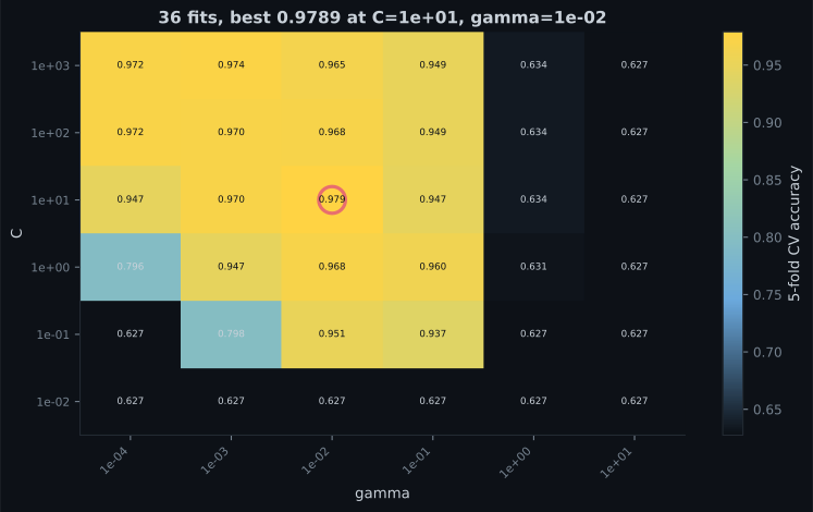
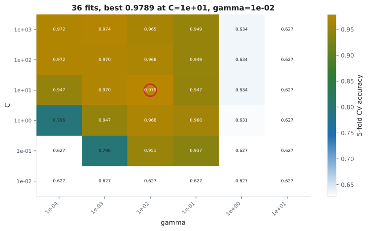
Section titled “Reading the plot”- The winner sits in a broad plateau, not on a spike. Several neighbouring cells score within 0.005 of the best. A winner on a spike would be suspicious — probably noise.
- Scores span 35 points. Hyperparameters are not a minor adjustment on this model; the wrong corner of the grid gives you a model barely better than guessing.
- The bad region is coherent. Large
gammawith smallCfails everywhere. Structure like that means the grid is telling you something about the model, not just about this dataset. - The best cell is interior. Neither
Cnorgammasits at a grid boundary, so the grid was wide enough — which is the check the next section is about.
See it move
Section titled “See it move”The search visits every cell in turn, keeping the best. Watch how much of the budget goes on the dark region — and how the running best stalls long before the last fit finishes.
Read the whole table
Section titled “Read the whole table”import pandas as pd
results = pd.DataFrame(search.cv_results_)
columns = ["param_svc__C", "param_svc__gamma", "mean_test_score",
"std_test_score", "rank_test_score"]
print(results[columns].sort_values("rank_test_score").head(5).to_string(index=False))
print()
print(f"best {results['mean_test_score'].max():.4f}")
print(f"worst {results['mean_test_score'].min():.4f}")
print(f"how many within 1% of the best: "
f"{(results['mean_test_score'] > results['mean_test_score'].max() - 0.01).sum()}")Three questions the table answers and best_params_ does not:
- Is the top score meaningfully above the runner-up? Compare the difference against
std_test_score. If the gap is smaller than the fold-to-fold spread, you picked between two equals. - Is the winner on a plateau or a spike? Plateau means robust; spike means you probably fitted noise.
- Did anything hit a grid boundary? If so, the grid was too narrow.
The edge-of-grid check
Section titled “The edge-of-grid check”def at_grid_edge(search, param_grid):
"""Warn when a chosen value sits at the boundary of its search range."""
edges = []
for name, values in param_grid.items():
values = list(values)
chosen = search.best_params_[name]
if len(values) > 1 and chosen in (values[0], values[-1]):
edges.append(f"{name}={chosen} is at the edge of {values[0]}..{values[-1]}")
return edges
for warning in at_grid_edge(search, param_grid):
print("WIDEN:", warning)A winner at the boundary means the search found the best value it was offered, and the true optimum may lie outside. Widen and rerun. Skipping this check is the most common way a grid search quietly under-delivers.
Tuning preprocessing too
Section titled “Tuning preprocessing too”The pipeline is a single estimator, so a grid can reach any step through the double-underscore
path — step__parameter, nested as deeply as needed:
from sklearn.compose import ColumnTransformer
from sklearn.impute import SimpleImputer
from sklearn.pipeline import Pipeline

pipe = Pipeline([
    ("pre", ColumnTransformer([("num", Pipeline([
        ("impute", SimpleImputer()),
        ("scale", StandardScaler()),
    ]), num_cols)])),
    ("model", SVC()),
])

param_grid = {
    "pre__num__impute__strategy": ["mean", "median"],   # preprocessing
    "pre__num__scale__with_mean": [True, False],        # preprocessing
    "model__C": [0.1, 1, 10],                           # model
    "model__gamma": [0.01, 0.1],                        # model
}
# 2 x 2 x 3 x 2 = 24 combinations
Whether to impute with the mean or the median is a hyperparameter exactly like C, and it should
be chosen the same way — by cross-validation, not by preference.
What tuning costs your honesty
Section titled “What tuning costs your honesty”Here is the uncomfortable part. best_score_ is the cross-validated score of the winning
combination — chosen because it scored highest on those same folds. It is the maximum of 36
noisy numbers, and the maximum of noisy numbers is biased upward.
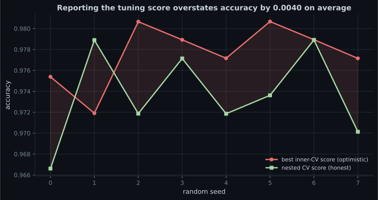
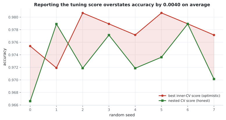
Nested cross-validation measures it. An outer loop holds out a fold; a complete grid search runs inside the remaining data; the winner is scored on the held-out fold. Selection never sees the rows it is judged on.
from sklearn.model_selection import GridSearchCV, KFold, cross_val_score

grid = {"svc__C": [0.1, 1, 10, 100], "svc__gamma": [1e-4, 1e-3, 1e-2, 1e-1]}

inner = KFold(4, shuffle=True, random_state=0)
outer = KFold(4, shuffle=True, random_state=100)

search = GridSearchCV(pipe, grid, cv=inner, n_jobs=-1)
search.fit(X, y)
print(f"tuning score (optimistic): {search.best_score_:.4f}")   # 0.9776 avg

nested = cross_val_score(search, X, y, cv=outer, n_jobs=-1)
print(f"nested score (honest):     {nested.mean():.4f}")        # 0.9736 avg
The cost is complete grid searches. Use nested CV when you need to report a number, and a plain search when you only need to choose a configuration — then report on a genuinely untouched test set.
Pitfalls
Section titled “Pitfalls”-
What separates a hyperparameter from a parameter?
Coefficients and split thresholds come out of fit(). C, max_depth and learning rate govern fit() itself, so no amount of fitting can choose them.
pch.quizShowAnswer
B — Parameters are learned by fitting; hyperparameters control how the fitting happens and must be chosen from outside it — Coefficients and split thresholds come out of fit(). C, max_depth and learning rate govern fit() itself, so no amount of fitting can choose them.
-
You have 4 hyperparameters with 5 values each and 5-fold CV. How many fits?
5 to the fourth is 625 combinations, times 5 folds is 3,125, plus one final refit on the whole training set.
pch.quizShowAnswer
D — 3,126 — 5 to the fourth is 625 combinations, times 5 folds is 3,125, plus one final refit on the whole training set.
-
Your grid search picks C = 1000, the largest value you offered. What should you do?
The search only ranks what it is given. A boundary winner is evidence the true optimum may lie outside the range.
pch.quizShowAnswer
B — Widen the grid — a winner at the boundary means the search found the best value it was offered, not the best value that exists — The search only ranks what it is given. A boundary winner is evidence the true optimum may lie outside the range.
-
Why does best_score_ overstate performance, and by how much here?
Taking the maximum of 16 noisy numbers biases the result upward. Nested CV separates selection from evaluation and measured a 0.9776 against 0.9736 gap.
pch.quizShowAnswer
B — It is the maximum of many noisy CV estimates, so selection bias inflates it — nested CV puts the overstatement at about 0.4 points on this problem — Taking the maximum of 16 noisy numbers biases the result upward. Nested CV separates selection from evaluation and measured a 0.9776 against 0.9736 gap.
🧪 Try It Yourself
Section titled “🧪 Try It Yourself”Exercise 1 – Count the fits before you run them
Section titled “Exercise 1 – Count the fits before you run them”Exercise 2 – Fit a grid search and read the winner
Section titled “Exercise 2 – Fit a grid search and read the winner”Exercise 3 – Read the whole results table
Section titled “Exercise 3 – Read the whole results table”Exercise 4 – Detect an edge-of-grid winner
Section titled “Exercise 4 – Detect an edge-of-grid winner”Exercise 5 – Measure the optimism with nested CV
Section titled “Exercise 5 – Measure the optimism with nested CV”- Parameters are fitted; hyperparameters govern the fitting and must be searched.
- Fits . Six hyperparameters at five values each is 78,125 fits.
- A list of grids avoids enumerating combinations that a kernel or solver ignores — 46 fits instead of 61 in the worked example.
- Log-space anything multiplicative:
C,gamma,alpha, learning rates. - Read
cv_results_, not justbest_params_. Here the grid spanned 0.6274 to 0.9789 and six cells tied within 1% of the top. - Check for an edge-of-grid winner every time.
best_score_is the maximum of many noisy numbers and overstates by about 0.4 points. Report a nested CV score or an untouched test set.
Exercise 6 – best_score_ is not the number you report
Section titled “Exercise 6 – best_score_ is not the number you report”Continue to RandomizedSearchCV for Large Parameter Spaces — when the grid has 78,125 combinations, sampling beats enumerating, and on this same problem it finds a better answer with the same budget.
pch.coffeeTagline
pch.coffeeCtapch.feedbackHeading
pch.feedbackSubheading