Cost Functions - Mean Squared Error (MSE)

What you’ll learn

• the difference between a cost function, a loss function and a metric
• the definition of MSE, and why we train on it but report RMSE
• how squaring changes what the model considers important
• MAE and Huber — what they optimise instead, and when each wins
• why the MSE surface is a convex bowl, and what that guarantees
• the statistical reason MSE is the default: it is maximum likelihood under Gaussian noise

Intuition

A model needs a single number that says how wrong it currently is — one number, because optimisation can only push one thing downhill. That number is the cost.

Choosing the cost is not a technicality. It is a statement of values. Squaring the errors declares that one miss of 10 is worse than ten misses of 1 (100 against 10), so the model will contort itself to avoid big misses even at the cost of many small ones. Taking absolute values declares they are equally bad. Both are defensible; they simply produce different models from identical data.

diagram Diagram mermaid

  flowchart LR
  X["Features X"] --> H["Model h(x)"]
  H --> P["Predictions ŷ"]
  Y["True targets y"] --> E["Errors ŷ - y"]
  P --> E
  E --> S["Square each one"]
  S --> M["Average → MSE"]
  M -->|"gradient"| H

Three words that get confused

Term	Scope	Example
Loss	One instance	$(\hat{y}_i - y_i)^2$
Cost	The whole training set — what the optimiser minimises	$\frac{1}{m}\sum(\hat{y}_i - y_i)^2$
Metric	What you report to humans; need not be differentiable	RMSE, MAE, $R^2$, “percentage within ±5%”

The cost and the metric are allowed to differ, and often should. You train on MSE because it has clean gradients; you report RMSE because it is in the units of the target.

The math

Definition

$$\text{MSE}(\boldsymbol{\theta}) = \frac{1}{m}\sum_{i=1}^{m}\left(\hat{y}^{(i)} - y^{(i)}\right)^2 = \frac{1}{m}\lVert \mathbf{X}\boldsymbol{\theta} - \mathbf{y}\rVert_2^2$$

Units are the square of the target’s units — squared dollars, squared degrees. Nobody has intuition for squared dollars, which is why we take the root:

$$\text{RMSE} = \sqrt{\text{MSE}}$$

Why train on MSE and report RMSE

The square root is monotonic, so whichever $\boldsymbol{\theta}$ minimises MSE also minimises RMSE. The minimiser is identical. But the gradient is not:

$$\frac{\partial}{\partial \theta_j}\text{MSE} = \frac{2}{m}\sum_i (\hat{y}^{(i)} - y^{(i)})x_j^{(i)}$$ $$\frac{\partial}{\partial \theta_j}\text{RMSE} = \frac{1}{2\sqrt{\text{MSE}}}\cdot\frac{\partial \text{MSE}}{\partial \theta_j}$$

The RMSE gradient carries a $1/\sqrt{\text{MSE}}$ factor that blows up as the cost approaches zero. MSE’s gradient is clean and linear in the residual. Same answer, better-behaved arithmetic — so train on MSE, report RMSE.

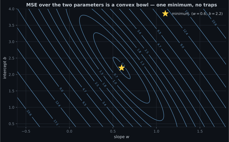
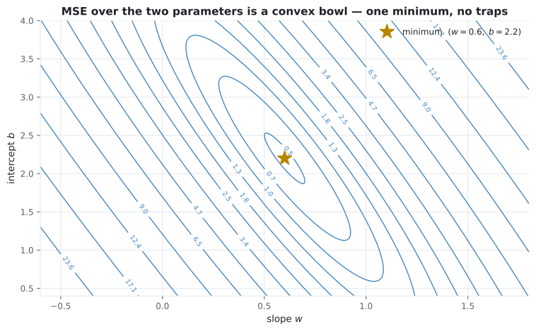
Why the surface is a bowl

$\text{MSE}(\boldsymbol{\theta})$ is a quadratic form in $\boldsymbol{\theta}$ with Hessian

$$\mathbf{H} = \frac{2}{m}\mathbf{X}^\top\mathbf{X}$$

$\mathbf{X}^\top\mathbf{X}$ is positive semi-definite for any $\mathbf{X}$ — for any vector $\mathbf{v}$, $\mathbf{v}^\top\mathbf{X}^\top\mathbf{X}\mathbf{v} = \lVert\mathbf{X}\mathbf{v}\rVert^2 \geq 0$. So the cost is convex: no local minima, no saddle points, no bad starting position. Whatever optimiser you point at it will find the global minimum, and if the columns are linearly independent that minimum is unique.

figure MSE over the two parameters of a simple linear model matplotlib

Nested ellipses closing on one point. Every direction leads downhill to the same place — this is what convexity looks like, and it is why linear regression never needs a restart.

Where this comes from

Convexity, Hessians and the second-derivative test are covered in Higher-Order Derivatives. The neural networks in the Deep Learning module have loss surfaces that are emphatically not convex — which is exactly why they need careful initialisation and momentum, and linear regression does not.

The statistical justification

MSE is not an arbitrary choice. Assume the target is a linear function plus Gaussian noise:

$$y^{(i)} = \boldsymbol{\theta}^\top\mathbf{x}^{(i)} + \varepsilon^{(i)}, \qquad \varepsilon^{(i)} \sim \mathcal{N}(0, \sigma^2)$$

The log-likelihood of the data is then

$$\log L(\boldsymbol{\theta}) = -\frac{m}{2}\log(2\pi\sigma^2) - \frac{1}{2\sigma^2}\sum_{i=1}^{m}\left(y^{(i)} - \boldsymbol{\theta}^\top\mathbf{x}^{(i)}\right)^2$$

Only the last term depends on $\boldsymbol{\theta}$, and it is $-\frac{1}{2\sigma^2}$ times the sum of squared errors. Maximising the likelihood is exactly minimising MSE. Choosing squared error is the same act as assuming your noise is Gaussian — which also explains why MSE handles outliers badly: Gaussians have thin tails and treat a large deviation as nearly impossible.

Worked example by hand

The Phase 3 five-point set with the fitted line $\hat{y} = 0.6x + 2.2$:

$x_i$	$y_i$	$\hat{y}_i$	$e_i$	$e_i^2$	$\lvert e_i \rvert$	Huber ($\delta=1$)
1	2	2.8	−0.8	0.64	0.8	0.32
2	4	3.4	+0.6	0.36	0.6	0.18
3	5	4.0	+1.0	1.00	1.0	0.50
4	4	4.6	−0.6	0.36	0.6	0.18
5	5	5.2	−0.2	0.04	0.2	0.02
				2.40	3.20	1.20

$$\text{MSE} = \frac{2.40}{5} = 0.48, \qquad \text{RMSE} = \sqrt{0.48} \approx 0.693, \qquad \text{MAE} = \frac{3.20}{5} = 0.64$$

Note that RMSE (0.693) exceeds MAE (0.64). That is not a coincidence: RMSE is always at least as large as MAE, and the gap widens as the errors become less uniform. A big RMSE-to-MAE ratio is a quick signal that a few large errors dominate.

Now break one point

Change the last observation from 5 to 25 and refit. The least-squares line becomes $\hat{y} = 4.6x - 5.8$:

$x_i$	$y_i$	$\hat{y}_i$	$e_i$
1	2	−1.2	+3.2
2	4	3.4	+0.6
3	5	8.0	−3.0
4	4	12.6	−8.6
5	25	17.2	+7.8

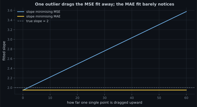
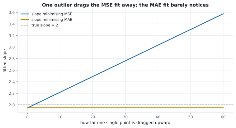
MSE has jumped from 0.48 to 30.88, and — far worse — every single point is now badly predicted. The line abandoned four good observations to chase one bad one. The MAE-optimal line for the same data is $\hat{y} \approx 1.51x + 0.49$, which stays close to the original four points and simply accepts a large error on the outlier.

Comparing the three losses

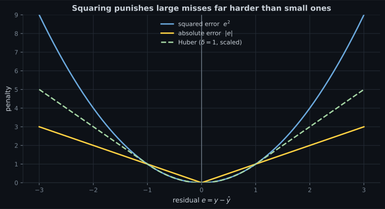
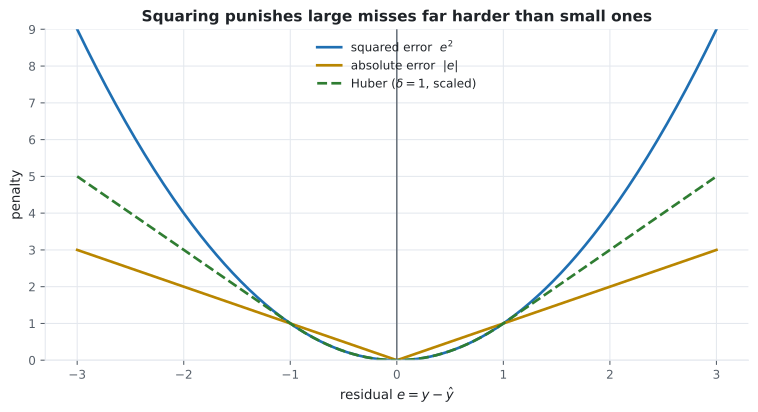
$$\text{MSE} = \frac{1}{m}\sum e_i^2 \qquad \text{MAE} = \frac{1}{m}\sum \lvert e_i \rvert \qquad \text{Huber}_\delta = \begin{cases} \tfrac{1}{2}e_i^2 & \lvert e_i\rvert \le \delta \\[4pt] \delta\left(\lvert e_i\rvert - \tfrac{1}{2}\delta\right) & \text{otherwise} \end{cases}$$

Huber is quadratic near zero (so it has a smooth gradient where it matters) and linear in the tails (so one wild point cannot dominate). It is the pragmatic default when you suspect outliers but still want gradient-friendly behaviour.

figure Penalty as a function of a single residual matplotlib

At a residual of 3 the squared loss charges 9 while absolute error charges 3. Huber tracks the parabola until the residual passes delta, then goes straight.

figure Dragging one point upward, and watching each loss react matplotlib

The MSE fit follows the outlier almost linearly. The MAE fit does not move at all — the median is immune to how far away the far point is.

Reading the plots

• The MAE line is flat. Not merely flatter — flat. Absolute-error fitting depends on the rank of the residuals, not their size, so once a point is above the line it does not matter whether it is above by 5 or by 500.
• The MSE line rises without limit. Each unit of extra distance adds a proportional pull on the slope. There is no point at which MSE stops caring.
• Huber sits between them, by construction. Below $\delta$ it behaves like MSE, above it like MAE, and $\delta$ is the dial.

	MSE	MAE	Huber
Optimises toward the	mean	median	mean, robustified
Outlier sensitivity	High	Low	Tunable via $\delta$
Differentiable everywhere	Yes	No (corner at 0)	Yes
Closed-form solution	Yes	No	No
scikit-learn	LinearRegression, Ridge	QuantileRegressor	HuberRegressor
Reach for it when	Noise is roughly Gaussian	Outliers are real data	You are unsure

MSE predicts the mean, MAE predicts the median

This is the deepest difference. The constant $c$ minimising $\sum(y_i - c)^2$ is the mean; the constant minimising $\sum\lvert y_i - c\rvert$ is the median. Everything else about their behaviour follows from that — including why MAE is the right loss when you care about the typical case and MSE when large errors are genuinely expensive.

See it move

Each pink square’s area is one point’s squared error. Watch the total area collapse as the line improves — that shrinking area is literally the cost.

sketch MSE as shrinking squares p5.js Pause Restart

Each square's area equals one point's squared error; as the fitted line improves, the squares shrink and MSE drops. Click for a fresh dataset.

From scratch

All three losses, plus the invariant that RMSE never falls below MAE:

losses.py

import numpy as np
 
 
def mse(y, pred):
    return float(((pred - y) ** 2).mean())
 
 
def rmse(y, pred):
    return mse(y, pred) ** 0.5
 
 
def mae(y, pred):
    return float(np.abs(pred - y).mean())
 
 
def huber(y, pred, delta=1.0):
    e = np.abs(pred - y)
    quadratic = 0.5 * e**2
    linear = delta * (e - 0.5 * delta)
    return float(np.where(e <= delta, quadratic, linear).mean())
 
 
x = np.array([1.0, 2.0, 3.0, 4.0, 5.0])
y = np.array([2.0, 4.0, 5.0, 4.0, 5.0])
pred = 0.6 * x + 2.2
 
print(f"MSE   = {mse(y, pred):.4f}")     # MSE   = 0.4800
print(f"RMSE  = {rmse(y, pred):.4f}")    # RMSE  = 0.6928
print(f"MAE   = {mae(y, pred):.4f}")     # MAE   = 0.6400
print(f"Huber = {huber(y, pred):.4f}")   # Huber = 0.2400
 
print(rmse(y, pred) >= mae(y, pred))     # True — always

With scikit-learn

robust_vs_ols.py

import numpy as np
from sklearn.linear_model import LinearRegression, HuberRegressor
from sklearn.metrics import mean_squared_error, mean_absolute_error
 
X = np.array([1.0, 2.0, 3.0, 4.0, 5.0]).reshape(-1, 1)
clean = np.array([2.0, 4.0, 5.0, 4.0, 5.0])
dirty = np.array([2.0, 4.0, 5.0, 4.0, 25.0])   # last point corrupted
 
ols_clean = LinearRegression().fit(X, clean)
ols_dirty = LinearRegression().fit(X, dirty)
huber_dirty = HuberRegressor(epsilon=1.35).fit(X, dirty)
 
print(f"OLS on clean data : slope {ols_clean.coef_[0]:.2f}")    # slope 0.60
print(f"OLS on dirty data : slope {ols_dirty.coef_[0]:.2f}")    # slope 4.60
print(f"Huber on dirty    : slope {huber_dirty.coef_[0]:.2f}")  # slope 1.91
 
# Same predictions, two different metrics
pred = ols_dirty.predict(X)
print(f"MSE = {mean_squared_error(dirty, pred):.2f}")           # MSE = 30.88
print(f"MAE = {mean_absolute_error(dirty, pred):.2f}")          # MAE = 4.64

One corrupted observation multiplies the OLS slope by more than seven, from 0.60 to 4.60. Huber still drifts — 1.91 — because five points is a brutal test and one of them is now an extreme value, but it absorbs less than half the damage OLS does.

Pitfalls

Do not compare MSE across datasets

MSE is in squared target units, so a house-price model and a temperature model produce numbers that cannot be compared. Even two models on the same target are only comparable if evaluated on the same rows. Use $R^2$ or a percentage error when you need a scale-free comparison.

A single terrible prediction can dominate the average

With 1,000 rows, one residual of 500 contributes 250,000 to the sum — more than 999 residuals of 15 combined. Always look at the error distribution, not just its mean. If RMSE is far above MAE, a handful of rows are doing all the damage.

Optimising a loss you do not care about

If the business cost of over-predicting differs from under-predicting, symmetric MSE is the wrong objective. Quantile regression (via QuantileRegressor, or loss="quantile" in gradient boosting) lets you weight the two directions differently.

MSE assumes Gaussian noise — check that

The maximum-likelihood derivation above is only valid for Gaussian errors. Heavy-tailed or skewed targets (income, insurance claims, waiting times) violate it badly. Log-transform the target, or switch to a loss matched to the actual distribution.

pch.quizTag pch.quizDefaultTitle

1. Why is MSE minimised during training while RMSE is reported afterwards?

   A They have different minimisers, and MSE's is better B They share the same minimiser, but MSE has a cleaner gradient while RMSE is in the target's units C RMSE cannot be computed during training D MSE is faster to compute than RMSE
   pch.quizShowAnswer

   B — They share the same minimiser, but MSE has a cleaner gradient while RMSE is in the target's units — The square root is monotonic, so the optimal parameters are identical. MSE's gradient is linear in the residual; RMSE's carries a 1 over root-MSE factor that explodes near zero.

2. Which constant value minimises the sum of absolute errors?

   A The mean B The median C The mode D The midpoint of the range
   pch.quizShowAnswer

   B — The median — The median minimises absolute error; the mean minimises squared error. That single fact explains most of the behavioural difference between MAE and MSE.

3. Why is the MSE cost surface guaranteed to have no local minima?

   A Because the learning rate is small enough B Because its Hessian, 2/m times X transpose X, is positive semi-definite, making the cost convex C Because the data is standardised D It is not guaranteed; local minima are common
   pch.quizShowAnswer

   B — Because its Hessian, 2/m times X transpose X, is positive semi-definite, making the cost convex — X transpose X is positive semi-definite for any X, so the quadratic cost is convex — a single global minimum with no traps along the way.

4. Your model reports RMSE 40 and MAE 12. What does that gap suggest?

   A A calculation error, since RMSE cannot exceed MAE by that much B A small number of very large errors are dominating the squared average C The model is underfitting everywhere equally D The target needs rescaling
   pch.quizShowAnswer

   B — A small number of very large errors are dominating the squared average — RMSE is always at least MAE, and the gap grows with the spread of the errors. A ratio above three points at a few extreme residuals rather than uniform mediocrity.

🧪 Try It Yourself

Exercise 1 – Compute MSE by hand

pch.exerciseTag pch.exerciseTitle

Exercise 2 – RMSE is never below MAE

pch.exerciseTag pch.exerciseTitle

Exercise 3 – Implement the Huber loss

pch.exerciseTag pch.exerciseTitle

Exercise 4 – Mean minimises MSE, median minimises MAE

pch.exerciseTag pch.exerciseTitle

Exercise 5 – Huber resists what OLS cannot

pch.exerciseTag pch.exerciseTitle

Recap

• Loss is per instance, cost is over the training set, and the metric is what you report.
• $\text{MSE} = \frac{1}{m}\sum e_i^2$; train on it, report RMSE because it is in target units.
• The cost surface is convex because $\mathbf{X}^\top\mathbf{X}$ is positive semi-definite — one global minimum, no traps.
• Minimising MSE is maximum likelihood under Gaussian noise, which is also why it fears outliers.
• MSE targets the mean, MAE the median, Huber the mean with a cap on how much any one point can pull.
• On the five-point set: MSE 0.48, RMSE 0.693, MAE 0.64, Huber 0.24. Corrupt one point and MSE jumps to 30.88 while the Huber slope barely moves.

Exercise 6 – Which statistic is each loss estimating?

pch.exerciseTag pch.exerciseTitle

Next

Continue to Gradient Descent Explained — how to actually walk down the bowl when the closed-form solution is too expensive to compute.