Intro to Convolutional Neural Networks (CNN) for Images

Every model so far flattened its input. Flattening a 28×28 image throws away the fact that pixel (5, 5) is next to pixel (5, 6) — and then asks the network to rediscover it from 784 unordered numbers. Convolution keeps that structure, and the saving is not subtle: on a 224×224 photo the first layer goes from 4,816,928 parameters to 896.

Every measurement on this page uses Fashion-MNIST — 28×28 greyscale clothing images, ten classes — because it is small enough to run every experiment on a CPU in seconds and real enough that the results mean something.

What you’ll learn

Convolution implemented in twelve lines and matched to tf.nn.conv2d at 2.38e−07.
What four hand-written kernels do to a real image, and why the kernel’s sum predicts its behaviour.
The parameter saving, counted: 78× on Fashion-MNIST, 5,376× on a 224×224 photo.
Receptive-field arithmetic: eight 3×3 layers see 17×17; add stride 2 and they see 511×511.
Output-shape arithmetic for valid and same padding at three strides, checked against Keras.
Equivariance verified: shifting the input shifts the feature map by exactly 0.00e+00 in the interior.

Convolution is a small weighted sum, repeated

A kernel is a small grid of weights. Slide it across the image, and at each position write down the sum of (kernel weight × pixel underneath):

\text{out}[i, j] = \sum_{u=0}^{k-1} \sum_{v=0}^{k-1} K[u, v] \cdot \text{in}[i + u, \; j + v]

The whole operation, no framework

def convolve(image, kernel):
    size = kernel.shape[0]
    out = np.zeros((image.shape[0] - size + 1, image.shape[1] - size + 1))
    for row in range(out.shape[0]):
        for column in range(out.shape[1]):
            patch = image[row:row + size, column:column + size]
            out[row, column] = (patch * kernel).sum()
    return out

On a 28×28 input with a 3×3 kernel that gives a 26×26 output — $28 - 3 + 1 = 26$ — and it costs 9 multiply-adds per output pixel, 6,084 for the whole map. Checked against tf.nn.conv2d: maximum difference 2.38e−07, which is float32 rounding.

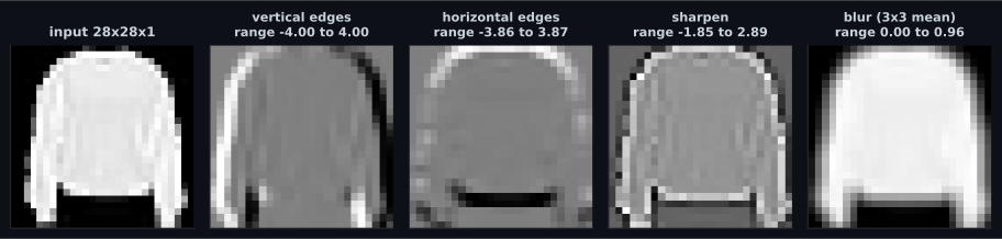
Five greyscale panels. The first is a 28x28 Fashion-MNIST pullover. The next four show the same image after a vertical-edge kernel, which highlights the left and right sides of the garment; a horizontal-edge kernel, which highlights the shoulders and hem; a sharpen kernel, which crisps the outline; and a 3x3 mean blur, which softens everything. — No training involved — these are four fixed grids of nine numbers each. The vertical-edge kernel responds to the garment's left and right boundaries and is near zero across the flat body; the horizontal one picks out the shoulders and hem instead. The two kernels whose weights sum to 1 preserve the image's overall brightness; the two that sum to 0 return zero wherever the input is flat.

Kernel	Sum of weights	Response range	Mean \|response\|
vertical edges	0.00	−4.0000 to 4.0000	0.7425
horizontal edges	0.00	−3.8627 to 3.8706	0.4515
sharpen	1.00	−1.8510 to 2.8941	0.8813
blur (3×3 mean)	1.00	0.0000 to 0.9617	0.6557

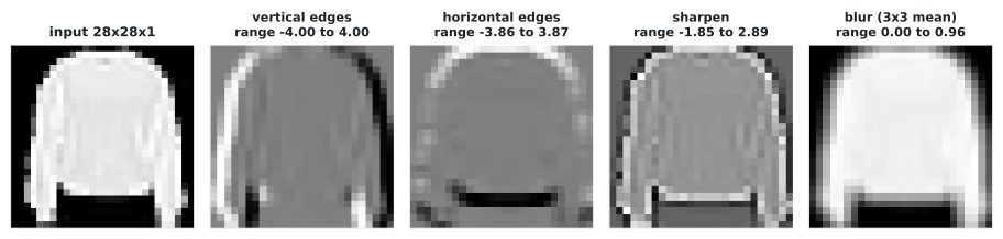
The sum of the weights tells you what a kernel is for. Sum to zero and it measures change: a flat patch produces exactly zero, so the output is an edge map. Sum to one and it preserves brightness: the blur’s output range (0.0000–0.9617) is nearly the input’s (0.0000–1.0000), because it is an average.

A convnet learns these numbers instead of being given them — but the first layer of a trained convnet reliably ends up looking like this set.

What it buys: parameters that do not depend on the image size

A Dense layer connects every input to every unit. A Conv2D layer connects a $k \times k$ window to every unit, and reuses the same weights at every position.

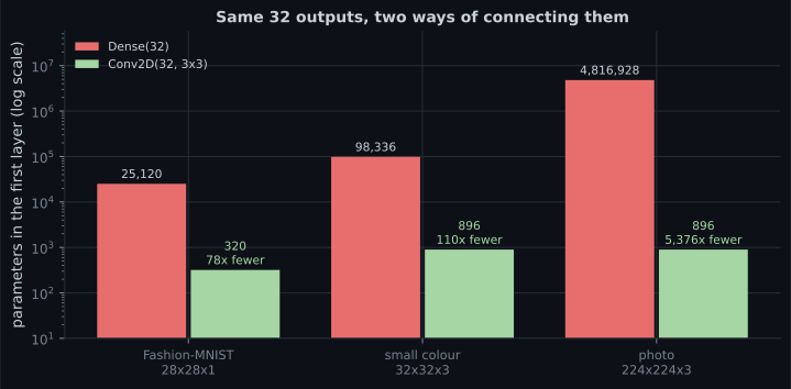
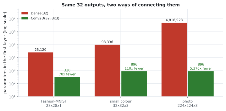
\text{Dense: } n_{\text{in}} \times u + u \qquad \text{Conv2D: } k^2 \times c_{\text{in}} \times c_{\text{out}} + c_{\text{out}}

Log-scale bar chart comparing Dense(32) against Conv2D(32, 3x3) for three input sizes. Dense grows from 25,120 to 98,336 to 4,816,928 parameters while Conv2D stays at 320, 896 and 896. — The Conv2D bars barely move: 320 parameters on a 28x28x1 input and 896 on a 224x224x3 one, because the count depends only on the kernel size and the channel counts. The Dense bars grow with the pixel count, reaching 4,816,928 on the photo — 5,376 times more for the same 32 outputs.

Input	`Dense(32)`	`Conv2D(32, 3×3)`	Ratio
Fashion-MNIST 28×28×1	25,120	320	78×
small colour 32×32×3	98,336	896	110×
photo 224×224×3	4,816,928	896	5,376×

Two properties fall out of weight sharing, and they are the reason convnets work on images:

The parameter count is independent of the input size. The same Conv2D(32, 3×3) layer handles 28×28 and 224×224 with 896 parameters, so a bigger image costs compute but not memory for weights.
A feature learned in one place works everywhere. A Dense layer would have to learn “vertical edge” separately for every position it might appear in.

diagram Diagram mermaid

  flowchart LR
  A["image
28x28x1"] --> B["Conv2D 32 filters 3x3
320 parameters"]
  B --> C["32 feature maps
28x28x32"]
  C --> D["downsample
14x14x32"]
  D --> E["Conv2D 64 filters 3x3
18,496 parameters"]
  E --> F["64 feature maps
14x14x64"]
  F --> G["global pooling
64 numbers"]
  G --> H["Dense 10
class scores"]
  I["the same weights are applied
at every position"] -.-> B

Each filter produces one feature map — a 2-D image of “how strongly this pattern responded here”. A layer with 32 filters produces 32 of them, stacked into a depth axis, and the next layer’s kernels span that whole depth: a 3×3 kernel over 32 channels is $3 \times 3 \times 32 = 288$ weights per filter.

Output shapes, exactly

Padding	Stride	Formula	Output side
`valid`	1	$\lceil (28 - 3 + 1)/1 \rceil$	26
`valid`	2	$\lceil (28 - 3 + 1)/2 \rceil$	13
`valid`	3	$\lceil (28 - 3 + 1)/3 \rceil$	9
`same`	1	$\lceil 28/1 \rceil$	28
`same`	2	$\lceil 28/2 \rceil$	14
`same`	3	$\lceil 28/3 \rceil$	10

Every row was checked against a real Conv2D layer. The trap is in the name: padding="same" does not mean “same output size” — it means “pad so the kernel can be centred on every input pixel”. With stride 1 that happens to preserve the size; with stride 2 it halves it.

Receptive fields: how deep is deep enough

Each layer’s output pixel depends on a small window of the layer below, which depends on a larger window below that. The recursion is

r_{\ell} = r_{\ell-1} + (k - 1) \cdot j_{\ell-1}, \qquad j_{\ell} = j_{\ell-1} \cdot s

where $r$ is the receptive field, $j$ the jump, $k$ the kernel size and $s$ the stride.

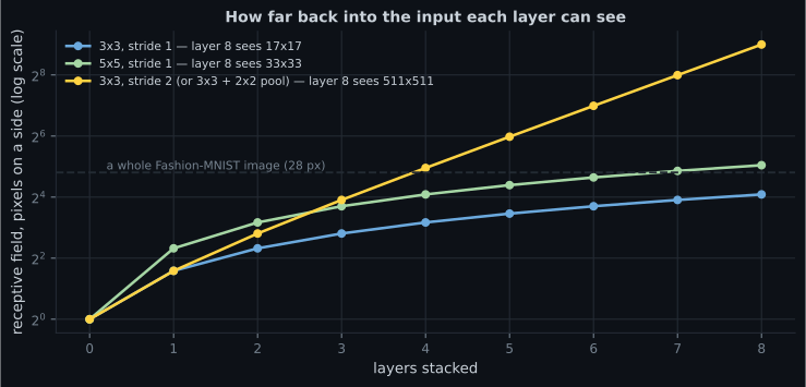
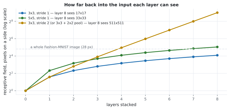
figure How far back into the input each layer can see matplotlib

With stride 1 the receptive field grows linearly — eight 3x3 layers reach 17 pixels, still less than a whole 28-pixel image. Introduce stride 2 and it grows geometrically, passing the image size by layer four and reaching 511 by layer eight. Downsampling is how convnets see globally without needing hundreds of layers.

Recipe	1 layer	2	4	8
3×3, stride 1	3	5	9	17
5×5, stride 1	5	9	17	33
3×3, stride 2	3	7	31	511
7×7, stride 1	7	13	25	49

Read the first two rows together: two 3×3 layers see the same 5×5 window as one 5×5 layer, using $2 \times 9 = 18$ weights per channel pair instead of 25 — and with a nonlinearity in between. That comparison is why almost every modern architecture is built from stacked 3×3 kernels.

Row three is why downsampling exists. Stride 1 alone would need dozens of layers before any unit could see a whole image.

Equivariance, and where it stops

Convolution commutes with translation: shift the input and the feature map shifts identically. Verified by shifting an image three pixels right and comparing against shifting the feature map three pixels right:

Region compared	max \|f(shift(x)) − shift(f(x))\|
the whole map	6.81e−01
the interior, excluding the border	0.00e+00

The interior agreement is exact. The whole-map discrepancy is entirely a boundary effect — the shift wraps pixels around the edge while padding="same" pads with zeros, so the two disagree only in the border columns. Stating this carelessly is a common error: convolution is exactly equivariant away from the boundary, and approximately equivariant at it.

Equivariance is not invariance. The feature map still knows where the object was:

Operation	max difference after a 3-pixel shift
global max pooling	1.07e−02
global average pooling	2.16e−02

Both are near zero but not zero — again from the boundary. Pooling over the whole map is what converts “the pattern is here” into “the pattern is present”, which is what a classifier needs.

sketch Slide a kernel by hand p5.js

A 3x3 kernel over an 8x8 input. Click a kernel, drag the highlighted window, and read the multiply-add that produces the output pixel.

sketch The measured table, ranked p5.js

Click a column to rank every row by it. The bars are that column's values and the highest and lowest are computed from the numbers, not written in.

Pitfalls

Reading padding="same" as “same output size”. With stride 2 it halves the side length; the name describes the padding, not the shape.
Forgetting that a kernel spans every input channel. A 3×3 kernel over 32 channels is 288 weights, not 9.
Stacking stride-1 layers and expecting global context. Eight of them see 17 pixels of a 28-pixel image. Downsample.
Claiming convolution is translation invariant. It is equivariant; pooling supplies the invariance.
Claiming equivariance is exact everywhere. Measured 0.00e+00 in the interior and 6.81e−01 at the boundary.
Choosing one 5×5 layer over two 3×3 layers. Same receptive field, 25 weights against 18, and one fewer nonlinearity.
Flattening straight after the last conv layer. That Dense layer will dominate the parameter count; global pooling usually works as well for far less.

Recap

Convolution is a small weighted sum slid across the input: 9 multiply-adds per output pixel, 6,084 for a 26×26 map, matched to TensorFlow at 2.38e−07.
A kernel’s weight sum predicts its behaviour: sum 0 measures change, sum 1 preserves brightness.
Weight sharing makes the parameter count independent of image size — 896 parameters on a 224×224×3 photo against 4,816,928 for Dense(32).
Output side is $\lceil (n - k + 1)/s \rceil$ for valid and $\lceil n/s \rceil$ for same, both checked against Keras.
Receptive field grows linearly with stride 1 (17 pixels after eight 3×3 layers) and geometrically with stride 2 (511).
Two 3×3 layers match one 5×5 layer’s receptive field with 18 weights instead of 25, plus an extra nonlinearity.
Convolution is exactly equivariant to translation in the interior (0.00e+00) and approximately so at the boundary; global pooling converts that into invariance.

Downsampling is the other half of the architecture, and there is more than one way to do it: Pooling & CNN Architecture.

pch.quizTag pch.quizDefaultTitle

A Conv2D(32, 3x3) layer has 896 parameters on a 224x224x3 input and 320 on a 28x28x1 one. Why does the image size barely matter?

pch.quizShowAnswer

B — Because the same kernel weights are reused at every position — the count is kernel area times input channels times filters, plus one bias per filter, with no dependence on the pixel count — Dense(32) on the same photo needs 4,816,928 parameters — 5,376 times more for the same 32 outputs.
You use Conv2D(32, 3, strides=2, padding='same') on a 28x28 input. What is the output side length?

pch.quizShowAnswer

B — 14 — 'same' pads so the kernel can be centred everywhere, but the stride still divides the output, giving ceil(28/2) — The name refers to the padding, not the output shape. With stride 1 it happens to preserve the size; with stride 2 it halves it.
Eight stacked 3x3 stride-1 layers have a receptive field of 17 pixels. What does that mean for a 28x28 image?

pch.quizShowAnswer

B — No unit can see the whole image yet, so a purely stride-1 stack needs many more layers — which is why downsampling exists, taking the field to 511 pixels by layer eight — With stride 2 the field grows geometrically and passes the image size by layer four.
Shifting an image 3 pixels right changed the feature map by 6.81e-01 over the whole map but 0.00e+00 in the interior. What does that show?

pch.quizShowAnswer

B — Convolution is exactly equivariant away from the boundary; the whole-map difference comes only from the edge, where a wrap-around shift and zero padding disagree — Precision matters here: the exact claim is interior equivariance. Boundaries always break it slightly, and so do stride and pooling misalignment.
Why do modern architectures prefer two stacked 3x3 layers over one 5x5 layer?

pch.quizShowAnswer

B — Because two 3x3 layers cover the same 5x5 receptive field using 18 weights per channel pair rather than 25, and add a nonlinearity in between — Same field, fewer weights, more nonlinearity. This is the observation VGG made and everything since has kept.

🧪 Try It Yourself

pch.coffeeTagline

pch.coffeeCta

pch.feedbackHeading

pch.feedbackSubheading