Framing an ML Problem & Getting the Data

What you’ll learn

the six questions that turn “predict house prices” into a specification you can build
how the downstream consumer of a prediction decides the model, not the other way round
RMSE versus MAE derived from $\ell_2$ and $\ell_1$ norms, and worked by hand on five districts
how to read a first histogram, and the four data-quality defects visible in this one
why “what does the current system do?” is the first question, not the last

Intuition

Most failed ML projects were never specified. Someone said “use machine learning on our housing data”, a model was trained, it scored well, and nobody could say what should happen next because nobody had asked what the number was for.

Framing is the work of turning a goal into a contract: what goes in, what comes out, who consumes it, and what counts as good enough. It costs an afternoon and saves months.

diagram Diagram mermaid

  flowchart TD
  A["Business goal
'know what districts are worth'"] --> B["Who consumes the output?"]
  B --> C["A downstream investment model
that takes a price estimate"]
  C --> D["Supervised regression
label = median house value"]
  D --> E["Performance measure
RMSE in dollars"]
  E --> F["Minimum acceptable
beat the current 15% error"]

The six framing questions

Ask these before writing a line of code. The answers for this phase’s running project are in the right column.

Question	Why it decides something	California housing
What is the business objective?	Determines what “good” means	Feed a district-level investment model
Who or what consumes the output?	Decides latency, format and units	Another model, in batch, overnight
What does the current solution do?	Sets the bar you must beat	Manual expert estimates, ~15% off
Is it supervised? What is the label?	Decides the whole method	Yes — `median_house_valuemedian_house_value`
Is it regression or classification?	Decides the model family and metric	Regression: a dollar amount
Is it batch or online?	Decides the serving architecture	Batch — data changes slowly

The third row is the one people skip. A model with 18% error looks respectable in isolation and is a regression against experts who manage 15%. Without that baseline number the project has no way to fail, which means it also has no way to succeed.

The math: choosing a performance measure

Both candidate measures are norms of the error vector, and the choice between them is the choice between two norms.

\text{RMSE}(\mathbf{X}, h) = \sqrt{\frac{1}{m}\sum_{i=1}^{m}\left(h(\mathbf{x}^{(i)}) - y^{(i)}\right)^2} \qquad \text{MAE}(\mathbf{X}, h) = \frac{1}{m}\sum_{i=1}^{m}\left\lvert h(\mathbf{x}^{(i)}) - y^{(i)}\right\rvert

RMSE is the $\ell_2$ norm of the error vector divided by $\sqrt{m}$ ; MAE is the $\ell_1$ norm divided by $m$ . More generally, the $\ell_k$ norm

\lVert\mathbf{v}\rVert_k = \left(\sum_i \lvert v_i\rvert^{k}\right)^{1/k}

weights large elements more heavily as $k$ grows. At $k = \infty$ only the single worst error counts. So the question “RMSE or MAE?” is really “how much extra should one badly wrong district cost me?”

Worked example by hand

Five districts, values in thousands of dollars:

district	actual $y$	predicted $\hat{y}$	error	$\lvert e\rvert$	$e^2$
1	200	210	+10	10	100
2	250	240	−10	10	100
3	300	310	+10	10	100
4	350	330	−20	20	400
5	400	500	+100	100	10,000
				150	10,700

\text{MAE} = \frac{150}{5} = 30 \qquad \text{RMSE} = \sqrt{\frac{10{,}700}{5}} = \sqrt{2140} \approx 46.26

The ratio is the signal. RMSE/MAE here is 1.54. If every error were the same size the ratio would be exactly 1; the further above 1, the more a few districts dominate. Report both and the ratio tells your reader something neither number does alone.

Which should you optimise? If the downstream investment model can absorb a few bad districts, MAE is the honest measure of typical performance. If one district valued at 500 when it is worth 400 triggers a bad investment, RMSE is correctly punishing the thing that hurts.

Two lines showing reported RMSE and MAE as a single district's error grows from 0 to 900 thousand dollars. RMSE climbs steeply and almost linearly; MAE rises only slightly. — Drag one error to $900k and RMSE nearly quintuples while MAE barely moves. Neither is wrong — they are answering different questions.

See it move

The five-district table is small enough to make interactive. Drag district 5’s prediction and watch both metrics — and their ratio — respond. Everything on screen is recomputed from the same five errors you are editing.

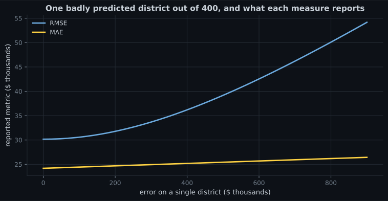
sketch One district, two metrics p5.js

Five districts with their predictions; drag the fifth prediction up or down. MAE tracks the error linearly while RMSE bends upward, and the RMSE/MAE ratio climbs away from 1 as the single error grows. Reset the drag and both metrics agree again.

Drag district 5 down to 410 and the errors become $+10, -10, +10, -20, +10$ : MAE 12.00, RMSE 12.65, ratio 1.054 — five comparable errors, two metrics that almost agree. Drag it up to 900 instead and MAE reaches 110.00 while RMSE reaches 223.92, ratio 2.035. One row moved, and the ratio doubled. That ratio is the answer to “is my error spread out or concentrated”, which is why reporting one metric without the other throws away information you already computed.

Getting the data

load_housing.py

import pandas as pd
 
URL = ("https://raw.githubusercontent.com/ageron/handson-ml2/master/"
       "datasets/housing/housing.csv")
 
housing = pd.read_csv(URL)
 
print(housing.shape)                    # (20640, 10)
print(housing["ocean_proximity"].value_counts())
# <1H OCEAN     9136
# INLAND        6551
# NEAR OCEAN    2658
# NEAR BAY      2290
# ISLAND           5
 
print(housing.info())
# total_bedrooms has 20433 non-null of 20640 -> 207 missing

load_housing.py

import pandas as pd
 
URL = ("https://raw.githubusercontent.com/ageron/handson-ml2/master/"
       "datasets/housing/housing.csv")
 
housing = pd.read_csv(URL)
 
print(housing.shape)                    # (20640, 10)
print(housing["ocean_proximity"].value_counts())
# <1H OCEAN     9136
# INLAND        6551
# NEAR OCEAN    2658
# NEAR BAY      2290
# ISLAND           5
 
print(housing.info())
# total_bedrooms has 20433 non-null of 20640 -> 207 missing

Three facts are already visible, and each one becomes a page of this phase:

total_bedroomstotal_bedrooms has 207 missing values → Data Cleaning
ocean_proximityocean_proximity is text, not a number → Handling Text & Categorical Attributes
ISLANDISLAND has five rows out of 20,640 — a random split can easily put zero of them in the training set → Creating a Test Set

Reading the first histogram

first_look.py

print(housing.describe().round(2))
 
housing.hist(bins=50, figsize=(12, 8))

first_look.py

print(housing.describe().round(2))
 
housing.hist(bins=50, figsize=(12, 8))

A three by three grid of histograms for median income, housing median age, total rooms, total bedrooms, population, households, latitude, longitude and median house value. Several are heavily right-skewed and two show a spike at their right edge. — Fifteen seconds of work, and it exposes a scaled unit, two hard caps, six right-skewed distributions and wildly different ranges.

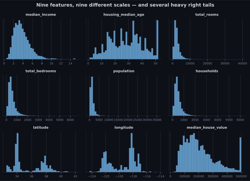
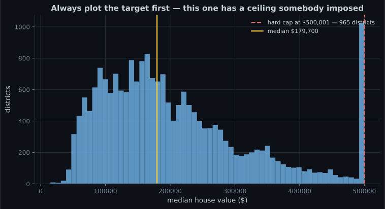
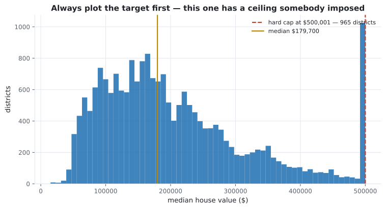
Reading the plot

median_incomemedian_income runs 0.4999 to 15.0001, not dollars. It has been scaled and capped, in units of tens of thousands. Nobody documents this; the histogram tells you.
housing_median_agehousing_median_age spikes at 52. 1,273 districts sit at exactly the maximum, because the value was clipped there.
median_house_valuemedian_house_value spikes at 500,001. 965 districts. This is the target, so the cap is a serious problem — see below.
Six distributions are strongly right-skewed. Some models care; a log transform is available if so.
Ranges differ by four orders of magnitude — median_incomemedian_income up to 15, populationpopulation up to 35,682. That is what Feature Scaling exists for.

Histogram of median house value showing a right-skewed distribution with a tall isolated spike at 500,001 dollars. — 965 districts share the identical value $500,001. The model will learn that no district is ever worth more, because in this data none ever is.

Pitfalls

quizCheck yourself

Why does 'who consumes the output' matter so much during framing?
Show answer
B — It determines latency, format, units, and whether errors will be noticed at all — a prediction feeding another model can be wrong for months without anyone knowing — A human reader spots an absurd number. A downstream model absorbs it and keeps producing plausible output from bad input, which is why pipeline consumers need monitoring.
Your model reports RMSE 46 and MAE 30. What does the ratio tell you?
Show answer
B — The errors are not uniform — a few large ones dominate the squared average — RMSE equals MAE only when every error is the same size. A ratio of 1.54 says the squared measure is being driven by a small number of large misses.
The target has 965 districts at exactly $500,001. What is the consequence?
Show answer
B — The model can never predict above that value, so it is invalid for expensive districts unless you get real labels or exclude them — A model cannot learn a relationship the labels do not contain. Either obtain proper labels for capped districts, or drop them and document the model's valid range.
What does a histogram of median_income running 0.4999 to 15.0001 tell you?
Show answer
B — The column has been scaled and capped — it is not raw dollars, and the units need to be established before anything is interpreted — Real incomes do not stop at 15. The column is in tens of thousands of dollars and clipped at both ends — the sort of thing a histogram reveals and a data dictionary often does not.

🧪 Try It Yourself

Exercise 1 – Compute both measures

Exercise 2 – Load the data and count categories

Exercise 3 – Find the missing values

Exercise 4 – Detect the caps

Exercise 5 – Establish the baseline to beat

Recap

Framing answers six questions: objective, consumer, current solution, supervision, task type, batch or online. Skipping the third leaves the project unable to fail or succeed.
RMSE is the $\ell_2$ norm of the errors, MAE the $\ell_1$ ; the choice encodes how much one bad district should cost.
Worked by hand: MAE 30, RMSE 46.26, ratio 1.54 — the ratio itself is diagnostic.
The dataset is 20,640 × 10, with 207 missing total_bedroomstotal_bedrooms and a five-row ISLANDISLAND category.
The first histogram exposes a scaled income column, a cap at age 52, and 965 districts pinned to the $500,001 target ceiling.
A capped target is a specification decision. Fix the labels, or state the model’s valid range.

Exercise 6 – Report the ratio, not just the metric

Continue to Creating a Test Set (Avoiding Data Snooping) — set data aside now, before exploring further, and see how much a purely random split distorts the strata you have just discovered.

If this helped you, consider buying me a coffee ☕

Buy me a coffee