
Inner Product of Functions
Everything so far treated a vector as a finite list of numbers, and every inner product as a finite sum. But nothing in Definition 3.3 mentions finiteness: an inner product needs to be bilinear, symmetric and positive definite, and that is all.
So take a function on an interval, think of it as a vector with one entry for every point of that interval, and replace the sum by an integral. All three axioms survive, and with them length, distance, angle and orthogonality. Two functions can now be perpendicular — and the family of functions that are mutually perpendicular in this sense is exactly the family Fourier analysis is built on.
What you’ll learn
Section titled “What you’ll learn”- Equation 3.37: the inner product of two functions as a definite integral, and why the interval is part of the definition.
- The book’s Example 3.9: and are orthogonal on , by exact cancellation rather than approximate smallness.
- The trigonometric family of Equation 3.38, measured to be orthogonal, with its Gram matrix computed.
- How a square wave is rebuilt from its projections, and why each coefficient can be computed independently of all the others.
- Parseval’s identity again, now predicting the truncation error exactly — and the Gibbs overshoot that will not go away.
Intuition: a vector with uncountably many entries
Section titled “Intuition: a vector with uncountably many entries”Sample a function at points and you get a vector in . Its dot product with another sampled function is . Multiply by the spacing and that sum is a Riemann approximation to .
Now let grow. The vector gets longer, the sum gets more terms, and the limit is the integral. The integral is the dot product of the two functions; the only difference is that the index set is a continuum instead of .
  flowchart TD
  FIN["finite vector
x ∈ ℝⁿ
⟨x,y⟩ = Σᵢ xᵢ yᵢ"]
  FIN --> SAMP["sample a function at n points
and it IS a finite vector"]
  SAMP --> LIM["let n → ∞, weight by Δx"]
  LIM --> FUN["⟨u,v⟩ = ∫ₐᵇ u(x) v(x) dx
Eq 3.37"]
  FUN --> A1["bilinear? yes — the integral is linear in each factor"]
  FUN --> A2["symmetric? yes — multiplication commutes"]
  FUN --> A3["positive definite? yes — ∫u² > 0 unless u ≡ 0"]
  A1 --> GEO["so length, distance, angle and
ORTHOGONALITY all carry over"]
  A2 --> GEO
  A3 --> GEO
  GEO --> ORTH["⟨sin, cos⟩ = 0 on [−π, π]
Example 3.9"]
  ORTH --> FOUR["{1, cos x, cos 2x, sin x, sin 2x, …}
is an orthogonal family — Eq 3.38
and that is the FOURIER basis"]
The math
Section titled “The math”Three things the notation hides.
The interval is part of the inner product. and are orthogonal on and not on , where . Changing changes the geometry exactly as changing the matrix did in §3.2.
Positive definiteness needs care. does not force at every point — a function that is zero except at one point still integrates to zero. The clean statement is that it forces almost everywhere, and the honest fix is to work in a space where functions differing on a measure-zero set are treated as the same vector. That is what means, and it is the only place in this chapter where the finite and infinite cases genuinely differ.
The integral must converge. Not every function pair has a finite inner product; on does not. The space of functions for which it does is the space you work in.
The induced norm and everything downstream
Section titled “The induced norm and everything downstream”Nothing new is being defined — these are §3.3 and §3.4 verbatim with the new inner product substituted in. That reuse is the point of having stated those sections abstractly.
The trigonometric family
Section titled “The trigonometric family”Their Gram matrix is diagonal rather than the identity, because these functions are orthogonal but not of unit length. Measured on the first seven members:
with every off-diagonal entry below . So this is an orthogonal basis, not an orthonormal one, and the coordinate formula needs the division that §3.5’s pitfall warned about:
Dividing by is not a convention plucked from nowhere — it is .
Worked example by hand
Section titled “Worked example by hand”Example 3.9 from the book
Section titled “Example 3.9 from the book”There are two ways to see that this is zero, and both are worth having.
By antiderivative. The double-angle identity gives , whose antiderivative is . So
By symmetry, which is the book’s argument and the better one. The product satisfies : it is odd. The integral of an odd function over an interval symmetric about the origin is zero, because every positive contribution on the right has an exactly equal negative partner on the left.
That is not “small”, it is cancellation. Measured, the positive area is and the negative area is — the same ten digits — and the integral comes out at exactly in floating point. The oddness itself is measured too: .
The square wave, by hand
Section titled “The square wave, by hand”Take on : on , on .
Coefficient on . Both and are odd, so their product is even and the integral is twice the right half:
Dividing by :
| for odd | measured | |
|---|---|---|
| 1 | ||
| 2 | — | |
| 3 | ||
| 4 | — | |
| 5 | ||
| 6 | — | |
| 7 |
The even coefficients are exactly , not small: for even , so the bracket is identically zero.
Coefficient on and on the constant. is odd and is even, so every product is odd and every one of those coefficients is zero. A square wave needs sines only, which is a statement about symmetry rather than about square waves.
import numpy as np

x = np.linspace(-np.pi, np.pi, 200001)          # odd count, so 0 is a sample
ip = lambda u, v: float(np.trapezoid(u * v, x))

# Example 3.9
w = np.sin(x) * np.cos(x)
print("<sin, cos>       =", f"{ip(np.sin(x), np.cos(x)):.3e}")
print("positive area    =", f"{float(np.trapezoid(np.where(w > 0, w, 0), x)):+.10f}")
print("negative area    =", f"{float(np.trapezoid(np.where(w < 0, w, 0), x)):+.10f}")
print("odd? max|w(x)+w(-x)| =", f"{np.max(np.abs(w + w[::-1])):.1e}")

# The Gram matrix of the first seven members of the trigonometric family.
fam = [("1", np.ones_like(x))]
fam += [(f"cos {k}x", np.cos(k * x)) for k in (1, 2, 3)]
fam += [(f"sin {k}x", np.sin(k * x)) for k in (1, 2, 3)]
G = np.array([[ip(a, b) for _, b in fam] for _, a in fam])
print("diagonal:", np.round(np.diag(G), 6))
print("largest off-diagonal:", f"{np.max(np.abs(G - np.diag(np.diag(G)))):.3e}")
print("2*pi =", round(2 * np.pi, 6), "  pi =", round(np.pi, 6))

# Square-wave coefficients, one independent integral each.
f = np.sign(np.sin(x))
print("||f||^2 =", round(ip(f, f), 6), " and 2*pi =", round(2 * np.pi, 6))
c = {k: ip(f, np.sin(k * x)) / ip(np.sin(k * x), np.sin(k * x)) for k in range(1, 8)}
print("coefficients:", {k: round(v, 6) for k, v in c.items()})
print("4/(k pi): ", {k: round(4 / (k * np.pi), 6) for k in (1, 3, 5, 7)})<sin, cos> = 0.000e+00
positive area = +0.9999999997
negative area = -0.9999999997
odd? max|w(x)+w(-x)| = 1.1e-15
diagonal: [6.283185 3.141593 3.141593 3.141593 3.141593 3.141593 3.141593]
largest off-diagonal: 4.441e-16
2*pi = 6.283185 pi = 3.141593
||f||^2 = 6.283185 and 2*pi = 6.283185
coefficients: {1: 1.27324, 2: -0.0, 3: 0.424413, 5: 0.254648, 4: -0.0, 6: -0.0, 7: 0.181891}See it move
Section titled “See it move”The first sketch is Example 3.9 with both frequencies on knobs. Set them equal and the cancellation stops.
The second sketch rebuilds the square wave one term at a time, and shows Parseval predicting the error.
The third sketch is the sum-to-integral limit, which is what justifies calling a function a vector.
From scratch
Section titled “From scratch”import numpy as np
def make_space(a, b, n=200001):
"""An inner product space of functions on [a, b], sampled for numerics."""
x = np.linspace(a, b, n)
def ip(u, v):
return float(np.trapezoid(u(x) * v(x), x))
def norm(u):
return np.sqrt(ip(u, u))
def angle_deg(u, v):
c = np.clip(ip(u, v) / (norm(u) * norm(v)), -1.0, 1.0)
return float(np.degrees(np.arccos(c)))
return x, ip, norm, angle_deg
x, ip, norm, angle = make_space(-np.pi, np.pi)
sin, cos = np.sin, np.cos
print("<sin, cos> on [-pi, pi]:", f"{ip(sin, cos):.3e}", " angle:", round(angle(sin, cos), 6))
print("||sin|| =", round(norm(sin), 6), " sqrt(pi) =", round(np.sqrt(np.pi), 6))
# The interval is part of the inner product.
_, ip2, norm2, angle2 = make_space(0.0, np.pi / 2)
print("<sin, cos> on [0, pi/2]:", round(ip2(sin, cos), 6),
" angle:", round(angle2(sin, cos), 4), "deg")
# Distance between two functions, and the triangle inequality on functions.
f = lambda t: np.sin(t)
g = lambda t: np.sin(t) + 0.3 * np.sin(3 * t)
h = lambda t: np.sin(t) + 0.3 * np.sin(3 * t) - 0.2 * np.cos(2 * t)
d = lambda p, q: norm(lambda t: p(t) - q(t))
print("d(f,g) =", round(d(f, g), 6), " d(g,h) =", round(d(g, h), 6), " d(f,h) =", round(d(f, h), 6))
print("triangle inequality holds:", d(f, h) <= d(f, g) + d(g, h) + 1e-12)<sin, cos> on [-pi, pi]: 0.000e+00 angle: 90.0
||sin|| = 1.772454 sqrt(pi) = 1.772454
<sin, cos> on [0, pi/2]: 0.5 angle: 50.4598 deg
d(f,g) = 0.531736 d(g,h) = 0.354491 d(f,h) = 0.639067
triangle inequality holds: TrueTwo results worth reading. On the angle between and is exactly ; on it is and the inner product is . Same two functions, different interval, different geometry — the interval plays precisely the role the matrix played in §3.2.
And , not . Sine is a unit vector under no particularly natural normalisation, which is why Fourier coefficients carry a .
On real data
Section titled “On real data”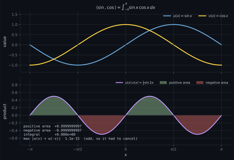
Reading the plot
Section titled “Reading the plot”From the cancellation figure. The green and red areas are visibly the same size, and the printed values agree to ten digits. That is what orthogonality of functions looks like: not a small residue but exact cancellation forced by symmetry.
The line to notice is the last one in the panel — . That is a check on the reason, not the result. The integral could be zero by accident; the product being odd is why it cannot be otherwise, and it is the argument the book gives.
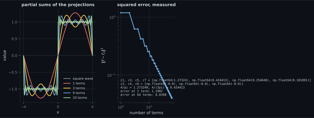
From the partial sums. Three separate things are measured here.
The coefficients match the closed form. against ; against ; against . And the even ones are exactly rather than , because the bracket is identically zero for even rather than nearly zero.
The error decays slowly, and Parseval says exactly how slowly. Measured: at one term, at three, at nine, at thirty-three, at sixty-four. That is roughly , which is bad as convergence rates go — and Parseval predicts it without running the approximation. The total energy is , and the energy captured by the first nine terms is . The difference is — exactly the measured error at nine terms.
That is §3.5’s Parseval identity doing predictive work: the truncation error is the energy you did not keep, and you can compute it from the coefficients without ever forming the approximation. It is the same statement as “the reconstruction error of a PCA truncation is the sum of the discarded eigenvalues”, which Chapter 10 will make.
The overshoot does not go away. The peak of the partial sum is at one term, at three, at nine, at thirty-three and at sixty-four. It is converging — to about , not to . This is the Gibbs phenomenon: near a jump discontinuity the partial sums overshoot by roughly of the jump, and adding terms makes the overshoot narrower without making it shorter.
Which is not a contradiction with convergence. The squared error does go to zero, because the region where the overshoot lives is shrinking. Convergence in the norm this page defines says nothing about convergence at any individual point — a distinction that matters the moment you use a truncated basis to reconstruct something with edges.
Pitfalls
Section titled “Pitfalls”Compare
Section titled “Compare”| finite vectors | functions on | |
|---|---|---|
| the vector | ||
| inner product | ||
| norm | ||
| dimension | infinite | |
| an orthogonal basis | eigenvectors, singular vectors | |
| coordinates | inner products | countably many integrals |
| truncation error | discarded squared coordinates | discarded squared coefficients |
| what can go wrong | conditioning | convergence, and pointwise behaviour |
The middle rows are identical in substance. The last row is where the two genuinely part company.
-
The book's argument that sin and cos are orthogonal on [-pi, pi] is not 'compute the antiderivative'. What is it?
Measured, the positive area is +0.9999999997 and the negative area -0.9999999997. The oddness is checked independently: the largest value of |w(x) + w(-x)| across the interval is 1.1e-15.
pch.quizShowAnswer
B — That their product is an odd function and the interval is symmetric about the origin, so every positive contribution has an exactly equal negative partner — Measured, the positive area is +0.9999999997 and the negative area -0.9999999997. The oddness is checked independently: the largest value of |w(x) + w(-x)| across the interval is 1.1e-15.
-
Why do Fourier coefficients carry a factor of 1/pi?
Measured, the Gram matrix of the first seven members is diag(6.283185, 3.141593, ...) with the largest off-diagonal entry at 4.4e-16. The factor-of-two difference on the constant term is a classic bug.
pch.quizShowAnswer
B — Because the trigonometric family is orthogonal but not orthonormal: the squared norm of sin kx is pi, so the coordinate formula divides by it — and the constant function, with squared norm 2pi, divides by 2pi instead — Measured, the Gram matrix of the first seven members is diag(6.283185, 3.141593, ...) with the largest off-diagonal entry at 4.4e-16. The factor-of-two difference on the constant term is a classic bug.
-
For the square wave, the measured squared error at nine terms is 0.253811. Where does that number also appear?
This is the same statement Chapter 10 makes about PCA: the reconstruction error of a truncation is the sum of the discarded squared coordinates. It lets you price a truncation without ever computing the approximation.
pch.quizShowAnswer
B — Parseval predicts it: the total energy is 2 pi = 6.283185 and the energy in the first nine coefficients is 6.029375, and the difference is 0.253811 exactly — the truncation error is the energy you did not keep — This is the same statement Chapter 10 makes about PCA: the reconstruction error of a truncation is the sum of the discarded squared coordinates. It lets you price a truncation without ever computing the approximation.
-
The peak of the partial sum converges to about 1.179 rather than to 1, while the squared error converges to zero. How are both true?
This is the Gibbs phenomenon: the overshoot is about nine percent of the jump and it gets narrower without getting shorter. Measured peaks: 1.273240 at one term, 1.182328 at nine, 1.179061 at sixty-four.
pch.quizShowAnswer
B — The overshoot occupies an ever-narrower region near the jump, so it contributes ever less to the integral — convergence in this norm says nothing about convergence at any individual point — This is the Gibbs phenomenon: the overshoot is about nine percent of the jump and it gets narrower without getting shorter. Measured peaks: 1.273240 at one term, 1.182328 at nine, 1.179061 at sixty-four.
🧪 Try It Yourself
Section titled “🧪 Try It Yourself”Exercise 1 – Reproduce Example 3.9 twice over
Section titled “Exercise 1 – Reproduce Example 3.9 twice over”Exercise 2 – The Gram matrix of the Fourier family
Section titled “Exercise 2 – The Gram matrix of the Fourier family”Exercise 3 – The interval changes the geometry
Section titled “Exercise 3 – The interval changes the geometry”Exercise 4 – Fourier coefficients, one integral each
Section titled “Exercise 4 – Fourier coefficients, one integral each”Exercise 5 – Parseval predicts the truncation error
Section titled “Exercise 5 – Parseval predicts the truncation error”Recall card
Section titled “Recall card”- The inner product of two functions is the integral of their product over an interval, Equation 3.37 — and the interval is part of the definition, not a detail.
- All three axioms survive, so length, distance, angle and orthogonality carry over unchanged from sections 3.3 and 3.4.
- Sine and cosine are orthogonal on the symmetric interval because their product is odd, so the positive and negative areas cancel exactly. The book’s argument is the symmetry, not the antiderivative.
- The trigonometric family is orthogonal but not orthonormal: squared norms are two pi for the constant and pi for every sine and cosine, which is where the one-over-pi in a Fourier coefficient comes from.
- Each coefficient is one independent integral, so adding a term never changes an earlier one — the same property an orthonormal basis has in finite dimensions.
- Parseval predicts the truncation error exactly: total energy minus the energy of the coefficients kept. Measured on a square wave at nine terms, both come to 0.253811.
- Convergence in this norm is not pointwise convergence. The Gibbs overshoot near a jump converges to about 1.179 rather than to 1, while the squared error still goes to zero, because the overshoot gets narrower rather than shorter.
- A function is a vector once you sample it, and the integral inner product is the limit of the finite dot product weighted by the spacing.
Next: Orthogonal Projections — the computation the whole chapter has been building towards.
pch.coffeeTagline
pch.coffeeCtapch.feedbackHeading
pch.feedbackSubheading