Introduction to Reinforcement Learning

The bandit page had one decision repeated a thousand times. Reinforcement learning proper adds the thing that makes it hard: actions change the situation you face next. A step towards the goal is also a step away from somewhere else, and a step into a pit ends the episode.

This page uses a gridworld small enough to solve exactly, which matters more than it sounds. Value iteration gives the true optimal policy, so every learned policy can be scored against the right answer rather than against a curve that merely goes up.

text

#########
#S.....G#     <- the short route: 6 steps, directly above the pits
#.XXXXX.#     <- pits: falling in ends the episode at -1
#.......#
#.......#     <- the long route: 12 steps, nowhere near the pits
#########

Actions succeed only 85% of the time — with probability 0.15 the agent moves somewhere else entirely. That single detail is what makes the short route a gamble rather than an obvious choice, and it is why the discount factor and the step cost below change the answer.

Policy	Mean reward	Mean steps	Reaches the goal	Takes the short route
Random	−1.0641	8.91	0.0075	0.7575
Q-learning (3,000 episodes)	0.5497	6.53	0.8025	0.9625
Value iteration (exact)	0.6568	13.32	0.8900	0.0775

Read the last column. The exact solution walks the long way round, and the agent that learned from experience did not — it found the shortcut, kept taking it, and ended up 0.1071 reward worse off with a goal rate 0.0875 lower.

What you’ll learn

The five pieces of an MDP, and why “solvable exactly” is the property that makes a teaching environment worth using.
What the discount factor actually decides — measured here as a switch between two routes.
What the step cost decides, measured the same way.
Why a learned policy that looks like it converged can still be worse than the optimum, and how to tell.

The pieces

An MDP is five things: states, actions, a transition rule, a reward, and a discount factor.

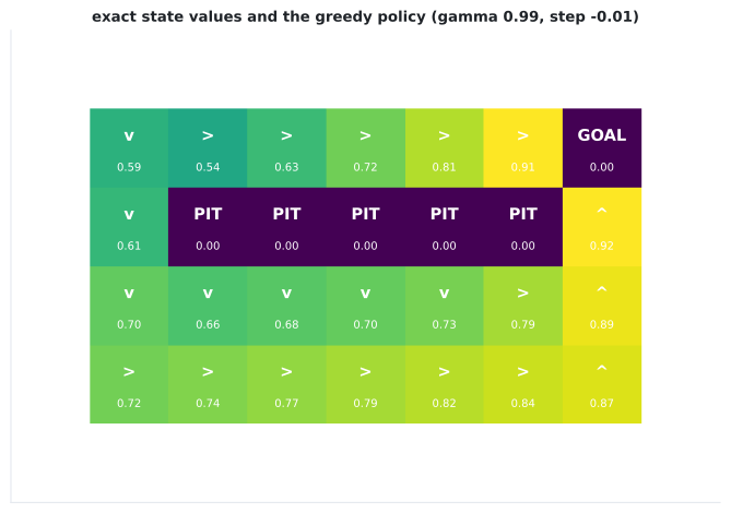
V^*(s) = \max_a \sum_{s'} P(s' \mid s, a)\left[R(s, a, s') + \gamma V^*(s')\right]

That is the Bellman optimality equation, and value iteration is what you get by treating it as an assignment and repeating it until nothing changes. On this world it converges in 29 sweeps to a start-state value of 0.5904.

Value iteration has to model the slip too

def backup(state, action, values, gamma):
    """Expected value of one action, over where it might actually land."""
    total = 0.0
    for candidate in range(4):
        probability = slip / 4 + (1.0 - slip if candidate == action else 0.0)
        following, reward, done = step(state, candidate)
        total += probability * (reward + (0.0 if done else gamma * values[following]))
    return total

The loop over candidate is the part that is easy to get wrong. If value iteration assumes the chosen action always happens, it computes the exact answer to a different problem — one without slip — and then confidently recommends the shortcut. An earlier version of this module did exactly that.

diagram Diagram mermaid

  flowchart LR
  S["state"] --> A["agent picks an action"]
  A --> E{"slip? 15%"}
  E -->|"85%: as intended"| N["next state"]
  E -->|"15%: a random action"| N
  N --> R["reward: -0.01 per step,
+1 goal, -1 pit"]
  R --> S
  N -.->|"short route"| P["6 steps, 0.79 goal rate"]
  N -.->|"long route"| Q["13 steps, 0.89 goal rate"]

Three policies

figure 400 evaluation episodes per policy matplotlib

The random policy reaches the goal 0.75% of the time — with pits adjacent to most of the map and a 15% slip, wandering ends badly fast, in 8.91 steps on average. Q-learning gets most of the way to the optimum and then stops: the dashed line it never reaches is the exact answer, and the gap is 0.1071 of reward.

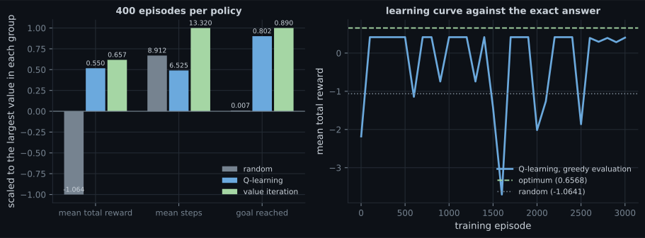
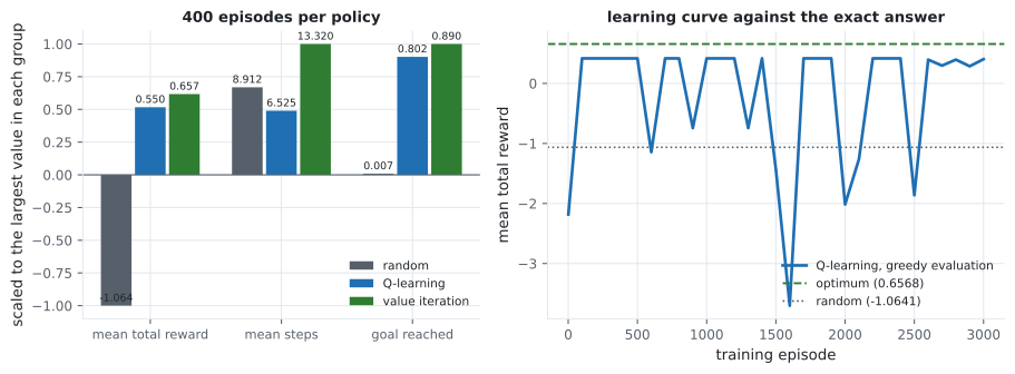
Q-learning’s failure here is worth being precise about, because “the curve went up” would have hidden it. Its policy takes the short route in 96.25% of episodes. The optimal policy takes it in 7.75%. Both reach the goal often; the shortcut just falls into a pit more.

The cause is exploration, not the update rule. ε-greedy at 0.1 finds the shortcut early, and from then on the long route is only ever visited by accident — a 12-step corridor requires a long run of exploratory actions to traverse, and each one is a coin flip. The agent never gathers enough evidence about a route it does not take. That is the bandit problem again, embedded in a world with states.

The discount factor decides the route

figure The optimal policy re-solved for each setting matplotlib

Both panels show the same trade from different directions. A low discount or an expensive step makes the distant pit penalty matter less than the immediate saving, so the optimal policy switches to the 6-step gamble — and the goal rate drops from 0.8900 to about 0.79 as a direct consequence. Nothing about the environment changed; only what the agent was told to value.

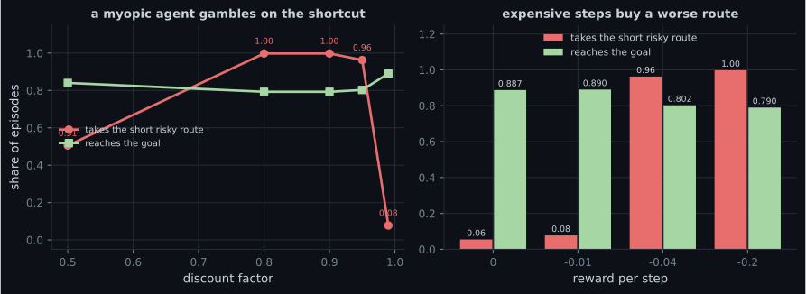
γ	Reward	Steps	Goal rate	Short route	Start value	Sweeps
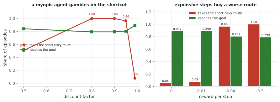
0.50	0.4641	22.59	0.8400	0.5050	−0.0223	21
0.80	0.5312	6.38	0.7925	0.9975	0.0983	21
0.90	0.5312	6.38	0.7925	0.9975	0.2625	23
0.95	0.5497	6.53	0.8025	0.9625	0.3914	26
0.99	0.6568	13.32	0.8900	0.0775	0.5904	29

Three things in that table are worth separating:

γ between 0.8 and 0.95 takes the gamble. The pit is several steps away, and at γ = 0.9 a penalty six steps ahead is worth $0.9^6 = 0.53$ of its face value. The shortcut’s risk is discounted; its saving is immediate.
γ = 0.99 takes the detour and is the only setting that reaches the goal 0.89 of the time.
γ = 0.50 is incoherent. It wanders for 22.59 steps and takes each route about half the time, because at that discount the goal itself is nearly worthless from the start state — the start value is negative (−0.0223). An agent that cannot see the reward cannot navigate towards it.

The step cost does the same job from the other end: free steps buy the safe detour (short route 0.0550), and steps costing 0.2 make the gamble worth it (0.9975), with the goal rate falling from 0.8875 to 0.7900.

The value map

figure Exact values and the greedy policy, gamma 0.99, step cost -0.01 matplotlib

This is what value iteration actually produces: a number per state, from which the policy falls out by taking the best action at each one. Note the arrows in the top row — even standing on the short route, the optimal action often points back down towards the safe corridor, because one slip above the pits ends the episode.

sketch Which route is worth it? p5.js

Drag the two sliders. The bars are the discounted value of each route under a simplified model of this world, and the verdict is which one that model prefers.

sketch The measured table, ranked p5.js

Click a column to rank every row by it. The bars are that column's values and the highest and lowest are computed from the numbers, not written in.

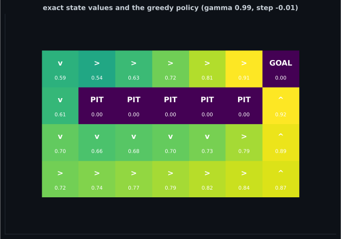
Pitfalls

Assuming a learned policy converged to the optimum. Q-learning here scored 0.5497 against 0.6568 and took a completely different route, after 3,000 episodes.
Modelling the environment’s randomness in the simulator but not in the solver. Value iteration must average over where an action might actually land, or its “exact” answer is exact for a different problem.
Treating the discount factor as a technical detail. It changed which route is optimal and moved the goal rate by 0.0975.
Using an environment with only one sensible route. An earlier version of this world had one, and every discount factor produced an identical policy — the sweep looked stable and measured nothing.
Reporting mean reward alone. Random scored −1.0641 with 8.91 mean steps, which sounds like a short efficient episode; it is a rapid fall into a pit.
Forgetting that the step cost is a design choice. It is not a physical fact about the world, and here it decides whether the agent gambles.

Recap

An MDP is states, actions, transitions, rewards and a discount; value iteration solves it exactly, in 29 sweeps on this world.
The world has a genuine trade-off — a 6-step route past the pits and a 12-step safe one — and slip at 15% is what makes it a trade-off at all.
The discount factor selects the route: γ ≤ 0.95 gambles (goal rate 0.7925), γ = 0.99 detours (0.8900).
The step cost selects it too: free steps → safe route, 0.2 per step → gamble.
Tabular Q-learning found the shortcut and stayed there, 96.25% against the optimum’s 7.75%, losing 0.1071 of reward — an exploration failure, not a learning-rule failure.
Random scored −1.0641 and reached the goal 0.75% of the time, which is the floor everything is measured against.

Q-learning’s failure here was about how it explored and how it updated. Both are tunable, and scaling the same update rule to a network needs two extra mechanisms: Q-Learning and Deep Q-Networks.

pch.quizTag pch.quizDefaultTitle

Value iteration takes the 13-step route while Q-learning takes the 6-step one 96.25% of the time. What went wrong?

pch.quizShowAnswer

B — Exploration — epsilon-greedy found the shortcut early, and traversing the 12-step safe corridor requires a long run of exploratory actions it almost never takes, so it never gathered evidence about the better route — The two policies were solved and learned with the same gamma. The gap is entirely about which experience the agent collected.
Why must value iteration average over the slip probability rather than assume the chosen action happens?

pch.quizShowAnswer

B — Because otherwise it computes the exact optimum for a deterministic world that does not exist — and that world's answer is to take the shortcut, since nothing can go wrong there — A solver and a simulator that disagree about the transition model produce a confident, wrong recommendation.
At gamma 0.90 the optimal policy takes the risky shortcut; at 0.99 it takes the safe detour. Why?

pch.quizShowAnswer

B — A discount shrinks distant outcomes — at gamma 0.9 a penalty six steps away is worth 0.53 of its face value, so the shortcut's immediate saving outweighs its discounted risk — The environment is identical in both cases. Only what the agent was told to value changed, and the goal rate moved 0.7925 to 0.8900 as a result.
At gamma 0.50 the agent wandered for 22.59 steps and the start state's value was negative (-0.0223). What does a negative start value mean here?

pch.quizShowAnswer

B — The discounted goal reward, seen from the start, is worth less than the accumulated step costs of getting there — so the agent has almost no signal pulling it towards the goal — It converged in 21 sweeps. A too-small discount makes distant rewards invisible, and an agent that cannot see the reward cannot navigate towards it.
The random policy scored -1.0641 with a mean of 8.91 steps. Why is the short episode length not a good sign?

pch.quizShowAnswer

B — It reached the goal only 0.75% of the time — the episodes are short because they end in a pit, which is exactly why reward and goal rate must be reported together — Steps-per-episode is only interpretable next to the outcome; a fast failure and a fast success look identical in that column alone.

🧪 Try It Yourself

pch.coffeeTagline

pch.coffeeCta

pch.feedbackHeading

pch.feedbackSubheading