Policy Gradients (Intro)

A DQN learns what each action is worth and picks the best one. REINFORCE skips that entirely: it adjusts the probability of each action directly, in proportion to how well the episode that contained it went.

\nabla_\theta J = \mathbb{E}\left[\sum_t \nabla_\theta \log \pi_\theta(a_t \mid s_t)\, G_t\right]

Read it as an instruction: make the actions you took more likely, weighted by the return that followed them. There is no value function, no replay buffer, no target network, and no maximum being taken over noisy estimates. In exchange there is one large new problem — the gradient is an average over whole episodes, and it is extremely noisy.

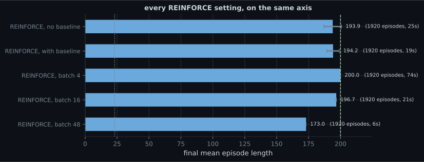
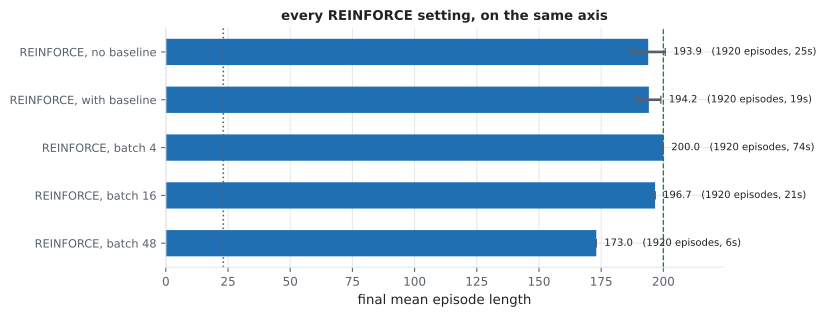
The standard fix is a baseline: subtract the mean return before weighting. Measured over three seeds on CartPole:

Setting	Final episode length	sd	Mean gradient norm
No baseline	193.91	6.86	1.6992
With baseline	194.18	4.80	0.0478

The baseline shrank the gradient norm by 35× and moved the final score by 0.27 — well inside the seed-to-seed spread. The variance reduction is real and easy to measure; its benefit on this task is not.

What you’ll learn

Why every raw return in CartPole is positive, and why that makes the estimator so noisy.
What a baseline actually changes — measured on the weights and on the gradient.
Why more, noisier updates beat fewer, cleaner ones at a fixed episode budget.
How REINFORCE compares with the DQN from the previous page, and what each one costs.

Every weight is positive

CartPole gives +1 per surviving step, so every discounted return is positive. That has a consequence people usually skip past:

Left: two overlapping histograms on separate axes — the raw discounted returns spanning roughly 1 to 30 and entirely positive, and the standardised weights centred on zero and spanning about -2 to 3. Right: mean gradient norm against episodes per gradient step, falling from 0.0810 at 4 episodes to 0.0497 at 48, with a second line showing final episode length falling from 200.00 to 173.04. — 100.0% of raw returns are positive, with mean 11.3202 and standard deviation 7.7908. Every action taken is therefore made MORE likely, and the only thing distinguishing a good action from a bad one is how much. After subtracting the mean and dividing by the spread, 45.1% of weights are negative — actions that did worse than average are now actively discouraged, which is a different learning signal entirely.

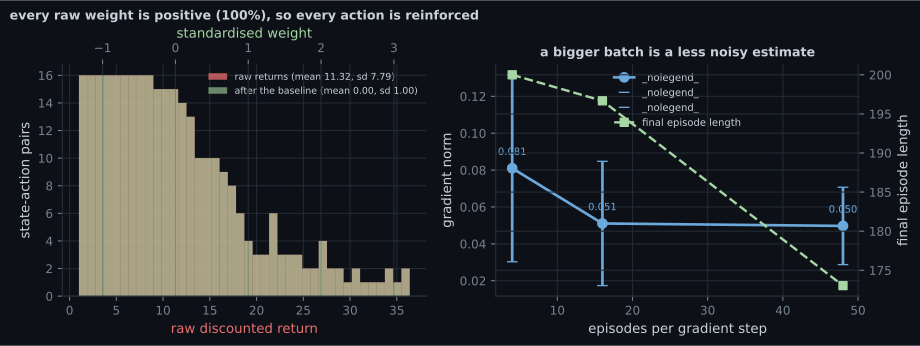
Without a baseline the update says “do more of everything, especially the things that happened in long episodes”. With one it says “do more of what beat the average, less of what didn’t”. The second is obviously better reasoning — and on this task it produced 194.18 against 193.91.

The baseline is two lines

weights = batch["weights"]                      # discounted returns
if baseline:
    weights = (weights - weights.mean()) / (weights.std() + 1e-8)

Subtracting a constant does not bias the gradient. The expected value of $\nabla_\theta \log \pi_\theta(a|s)$ is zero, so subtracting any quantity that does not depend on the action leaves the expectation unchanged while reducing the variance. Dividing by the standard deviation does change the effective learning rate, which is why the measured gradient norm falls so far.

The baseline, measured

Left: learning curves against episodes of experience for three seeds each with and without a baseline, all rising from about 20 towards the 200 cap with the baseline runs slightly tighter together. Right: bars of final episode length for the two settings, nearly identical at 193.91 and 194.18, next to bars of mean gradient norm showing 1.6992 against 0.0478. — Both settings solve CartPole — the environment caps episodes at 200 and both land within 6 of it. The gradient norms differ by a factor of 35, which is the variance reduction the theory promises, but that reduction had nowhere to show up in the score because the task was already being solved. The seed spread narrowed slightly, 6.86 to 4.80, which is the only visible benefit and is not significant with three seeds.

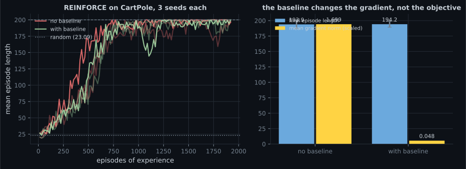
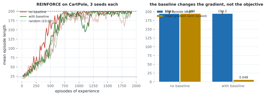
This is a case where the honest reading needs stating plainly: the mechanism worked and the outcome did not move. The baseline demonstrably did what it is supposed to do to the gradient. CartPole with a 200-step cap simply is not hard enough for that to matter — both configurations reach the ceiling. On a longer or sparser task the same 35× reduction would be the difference between learning and not.

Reporting “the baseline improved the score” here would have been false; reporting “the baseline does nothing” would be equally false.

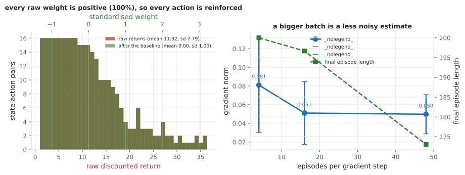
Smaller batches won

The batch size is how many complete episodes go into one gradient. Bigger batches average more episodes, so the estimate is less noisy. Holding the total experience fixed at 1,920 episodes:

Episodes per step	Updates	Final length	Gradient norm	Norm sd
4	480	200.00	0.0810	0.0507
16	120	196.68	0.0510	0.0337
48	40	173.04	0.0497	0.0210

The gradient does get cleaner with a bigger batch — norm sd falls from 0.0507 to 0.0210, exactly as expected. And performance gets worse, from a perfect 200.00 down to 173.04.

At a fixed budget, batch size trades update count against update quality, and here the count mattered more. Four episodes per step gives 480 chances to improve the policy; 48 episodes gives 40. A noisy step in roughly the right direction, taken twelve times, beat one clean step.

That is not a universal law — it is what this budget and this task produced. The general lesson is that “reduces variance” and “learns better” are separate claims needing separate measurements, which is the same conclusion the baseline section reached by a different route.

diagram Diagram mermaid

  flowchart TD
  E["collect complete episodes"] --> R["discounted return per step"]
  R --> B{"baseline?"}
  B -->|"no"| P["all weights positive
norm 1.6992"]
  B -->|"yes"| N["45.1% negative
norm 0.0478"]
  P --> G["one gradient step"]
  N --> G
  G --> S{"batch size at fixed budget"}
  S -->|"4 episodes, 480 updates"| W["200.00"]
  S -->|"48 episodes, 40 updates"| L["173.04"]

figure Every configuration on one axis matplotlib

All five settings solve the task to some degree — the worst is 173.04 against a random baseline of 23.09. The spread between them is the interesting part, and it is driven by update count rather than by gradient quality: the configuration with the noisiest gradients (batch 4, norm sd 0.0507) reached the cap exactly.

REINFORCE against DQN

Both were run on the same CartPole with the same 200-step cap:

Algorithm	Best measured score	What it needs
DQN (replay + target)	144.20	A replay buffer, a target network, and both are required
REINFORCE (batch 4)	200.00	Complete episodes before any update

REINFORCE won here, and the comparison deserves two caveats rather than a victory lap. First, REINFORCE consumed 1,920 complete episodes while the DQN used 6,000 frames across 16 environments — different budgets in different units, so this is not a sample-efficiency result. Second, REINFORCE’s advantage is partly that CartPole’s episode-return signal is dense and well-shaped; on a task with sparse rewards the value-based approach has structure that REINFORCE lacks.

What is fair to conclude: REINFORCE is dramatically simpler to implement — no buffer, no target network, no ablation needed to make it work — and on a short, dense-reward task that simplicity costs nothing.

sketch Why the baseline matters p5.js

Drag the slider to move the baseline. The bars are per-action weights from a batch of episodes; green pushes the action's probability up, red pushes it down.

sketch The measured table, ranked p5.js

Click a column to rank every row by it. The bars are that column's values and the highest and lowest are computed from the numbers, not written in.

Pitfalls

Claiming a baseline improved the score without measuring. Here it changed the final result by 0.27 while shrinking the gradient norm 35×.
Assuming a cleaner gradient learns better. The noisiest configuration (batch 4) scored 200.00; the cleanest (batch 48) scored 173.04 on the same experience.
Comparing algorithms on different budgets. REINFORCE used 1,920 episodes and the DQN 6,000 frames across 16 environments; those units are not interchangeable.
Updating before an episode finishes. REINFORCE weights each action by the return that followed it, so the episode must complete first.
Collecting episodes one at a time. Running 16 in a vectorised environment costs one model call per timestep instead of one per timestep per episode — measured at roughly 16× faster.
Forgetting that dividing by the standard deviation changes the step size. It is a normalisation, not just a recentring, and it interacts with the learning rate.

Recap

REINFORCE adjusts action probabilities directly, weighted by the return that followed each action — no value function, no replay, no target network.
Every CartPole return is positive (100.0% of them), so without a baseline every action taken is reinforced and only the magnitude differs.
A baseline made 45.1% of weights negative and cut the gradient norm from 1.6992 to 0.0478, a 35× reduction, with no measurable change in final score on this task.
At a fixed 1,920-episode budget, 4 episodes per update scored 200.00 and 48 scored 173.04 — update count beat update quality.
REINFORCE’s best (200.00) exceeded the DQN’s best (144.20) here, on a different budget and a task that suits it.
“Reduces variance” and “learns better” are separate claims and need separate measurements.

A baseline that cut the gradient norm 35x and moved the score by 0.27 is an odd place to stop. The next page replaces it with a learned critic, then attacks a different axis entirely and gets a 3.2x sample-efficiency win out of it: Actor-Critic and PPO (Intro).

pch.quizTag pch.quizDefaultTitle

In CartPole, 100% of the raw discounted returns are positive. What does that imply for REINFORCE without a baseline?

pch.quizShowAnswer

B — Every action taken is made more likely, and the only thing separating good from bad actions is how much — which is a much weaker and noisier signal than pushing bad actions down — Subtracting the batch mean made 45.1% of the weights negative, turning 'do more of everything' into 'do more of what beat the average'.
A baseline reduced the mean gradient norm from 1.6992 to 0.0478 but changed the final score from 193.91 to 194.18. What is the honest conclusion?

pch.quizShowAnswer

B — The variance reduction is real and measurable, but this task was already being solved to the 200-step cap, so there was no room for it to show up in the score — Both readings — 'it improved the score' and 'it does nothing' — would be false. The mechanism worked; the outcome had no headroom.
At a fixed budget of 1,920 episodes, 4 episodes per update scored 200.00 and 48 per update scored 173.04, while the gradient noise fell with batch size. Why?

pch.quizShowAnswer

B — Batch size trades update count against update quality at a fixed budget — 4 episodes bought 480 updates against 40, and many roughly-right steps beat a few precise ones here — The measured gradient norm sd did fall from 0.0507 to 0.0210, confirming the cleaner estimate. It simply was not what limited learning.
Why must REINFORCE wait for an episode to finish before updating?

pch.quizShowAnswer

B — Because each action is weighted by the discounted return that followed it, which is not known until the episode ends — This is the structural difference from Q-learning, which bootstraps from its own estimate of the next state and can update after a single transition.
REINFORCE reached 200.00 while the DQN reached 144.20 on the same environment. What can be concluded?

pch.quizShowAnswer

B — Not much beyond this setup — the two used different budgets in different units, and CartPole's dense episode-return signal happens to suit REINFORCE — REINFORCE consumed 1,920 complete episodes while the DQN used 6,000 frames across 16 environments; the fair claim is about implementation simplicity, not sample efficiency.

🧪 Try It Yourself

pch.coffeeTagline

pch.coffeeCta

pch.feedbackHeading

pch.feedbackSubheading