Advanced Recurrent Layers (Dropout, Stacking, Bidirectional)

A single LSTM(32) on 5,000 IMDB reviews scores 0.8260. Three refinements are the standard next moves: regularise it, stack it, run it in both directions. All three were measured here on the identical model, data and seed, at eight epochs.

Change	Best validation accuracy	Against the baseline	Seconds
baseline LSTM(32)	0.8260	—	129.5
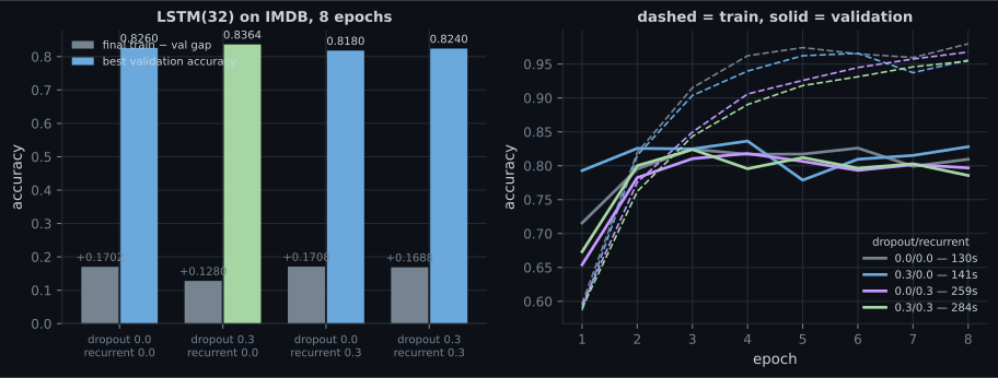
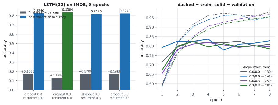
dropout=0.3	0.8364	+0.0104	141.3
recurrent_dropout=0.3	0.8180	−0.0080	259.2
both at 0.3	0.8240	−0.0020	284.3
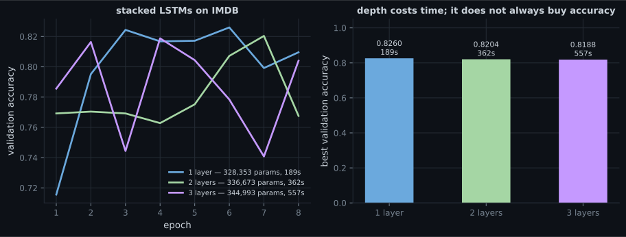
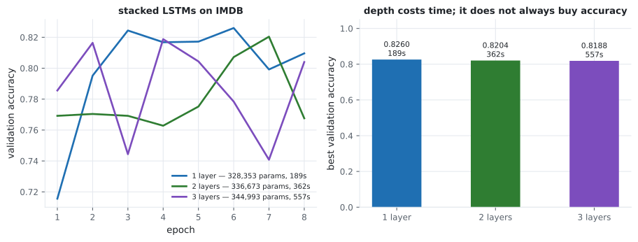
2 stacked layers	0.8204	−0.0056	362.5
3 stacked layers	0.8188	−0.0072	557.4
Bidirectional (32+32)	0.8448	+0.0188	225.3
Bidirectional (16+16, matched width)	0.8284	+0.0024	262.7

One of the three helped. One cost twice the wall-clock to lose accuracy. One helped mostly because it doubled the model’s width.

What you’ll learn

• The difference between dropout and recurrent_dropout — different tensors, different masks, very different cost.
• Why recurrent_dropout doubled the training time: it drops off TensorFlow’s fused kernel.
• The return_sequences rule that makes stacking possible, and why depth lost here.
• What Bidirectional actually costs, and how to tell a real gain from a width gain.
• The one setting a forecaster must never use, and the leak that makes it look good.

Two dropout arguments, two different tensors

$$\begin{aligned} h_t &= f\!\left(W_x \cdot (\underbrace{m_x \odot x_t}_{\texttt{dropout}}) + W_h \cdot (\underbrace{m_h \odot h_{t-1}}_{\texttt{recurrent\_dropout}}) + b\right) \end{aligned}$$

• dropout masks the input $x_t$ at each step.
• recurrent_dropout masks the previous state $h_{t-1}$ — inside the loop.

Both use the same mask at every timestep (a “variational” mask). That matters: a fresh mask per step would resample the noise 200 times along one sequence and destroy anything the state was carrying. A Dropout layer placed between two recurrent layers does exactly that resampling — which is fine there, because it sits outside the recurrence.

figure LSTM(32) on IMDB, 8 epochs, four dropout settings matplotlib

Plain dropout is the only setting that did what dropout is for: it cut the train-validation gap from 0.1702 to 0.1280 and gained 0.0104 accuracy. Recurrent dropout barely moved the gap (0.1708) and lost 0.0080 while costing twice the wall-clock. The dashed curves show why the gap is worth watching separately from the score: every one of these models is memorising the training set by epoch 5.

The cost nobody mentions

recurrent_dropout took 259.2 seconds against 129.5 — exactly 2.0×. The reason is implementation, not mathematics: cuDNN and TensorFlow’s fused CPU kernels implement the whole recurrence as one optimised operation, and applying a dropout mask inside the loop forces Keras to fall back to the generic step-by-step path.

The same is true of mask_zero=True, which every page in this phase uses. The two together are why this module was the slowest in the phase.

Setting	Fused kernel	Measured cost
plain LSTM	yes	1.0×
dropout=0.3	yes	1.1×
recurrent_dropout=0.3	no	2.0×

If you want regularisation and speed, use dropout plus a Dropout layer after the recurrent layer, and reach for recurrent_dropout only when the gap says you need it.

Stacking

Every recurrent layer except the last needs return_sequences=True, or the next one receives a vector where it expects a sequence:

A two-layer stack

model = keras.Sequential([
    keras.layers.Input((200,)),
    keras.layers.Embedding(10000, 32, mask_zero=True),
    keras.layers.LSTM(32, return_sequences=True),    # (batch, 200, 32)
    keras.layers.LSTM(32),                           # (batch, 32)
    keras.layers.Dense(1, activation="sigmoid"),
])

figure Stacked LSTMs on IMDB matplotlib

Depth cost accuracy monotonically and time linearly: each extra layer added 8,320 parameters, roughly 180 seconds, and lost about 0.006 accuracy. Sentiment on 5,000 reviews does not have a hierarchy of temporal features for a second layer to build on — the first layer already extracts everything the task needs, and the second only adds optimisation difficulty.

Layers	Parameters	Best validation accuracy	Seconds
1	328,353	0.8260	188.8
2	336,673	0.8204	362.5
3	344,993	0.8188	557.4

Stacking is genuinely useful when the task has structure at several timescales — speech (phonemes → words), music, long documents. It is not a general-purpose capacity dial, and on this task it was a pure loss: 3× the training time for −0.0072 accuracy.

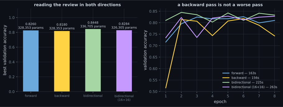
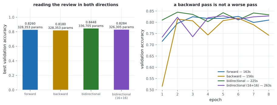
Bidirectional

Bidirectional runs two copies of the layer — one forward, one over the reversed sequence — and concatenates their outputs. Reading a review backwards is not a worse way to read it: the backward model alone scored 0.8180 against the forward model’s 0.8260.

figure Forward, backward, and both matplotlib

The naive reading is that Bidirectional bought +0.0188. The matched-width control says otherwise: two 16-unit directions, which cost slightly fewer parameters than one 32-unit forward layer, gained only +0.0024. Most of the headline win was the extra width, not the extra direction — and the backward-only run's first epoch at 0.52 is a reminder that the two directions are not interchangeable during optimisation even when they end up equivalent.

Setup	Parameters	Best validation accuracy	Against forward
forward LSTM(32)	328,353	0.8260	—
backward LSTM(32)	328,353	0.8180	−0.0080
Bidirectional(LSTM(32))	336,705	0.8448	+0.0188
Bidirectional(LSTM(16))	326,305	0.8284	+0.0024

Always include the matched-width control. Any wrapper that doubles a layer’s output width will look good against the un-doubled version; the question is whether the structure helped, and here it was worth 0.0024, not 0.0188.

diagram Diagram mermaid

  flowchart TB
  A["is the train-validation gap large?"] -->|"no"| B["regularisation will not help
— add capacity or data"]
  A -->|"yes"| C["dropout=0.3
+0.0104, gap 0.1702 → 0.1280"]
  C --> D{"still overfitting?"}
  D -->|"yes"| E["recurrent_dropout
— but it costs 2.0x wall-clock"]
  D -->|"no"| F["done"]
  G["is the task hierarchical
in time?"] -->|"yes"| H["stack, with
return_sequences=True"]
  G -->|"no"| I["one layer
— depth lost 0.0072 here"]
  J["will the whole sequence
exist at prediction time?"] -->|"yes"| K["Bidirectional
— check matched width"]
  J -->|"no (forecasting)"| L["forward only
— the backward pass reads the future"]

The one that is a bug, not a trade-off

For classification, Bidirectional is a legitimate choice: the whole review exists before you classify it. For forecasting, it is a leak. The backward pass at timestep $t$ has consumed timesteps $t+1 \ldots T$, and at prediction time those have not happened.

The failure mode is nasty because it validates beautifully. Your offline metric improves, because your offline data contains the future; production then fails silently. Exercise 5 demonstrates it directly: on a task where the answer sits at the last timestep and must be reported from the first, a forward model cannot exceed chance and a bidirectional one solves it.

The same reasoning covers every “look-ahead” mistake in the phase — shuffled splits, scalers fitted on all the data, and target-derived features.

sketch Which timesteps has each direction seen? p5.js Pause Restart

Move the query step and watch what the forward, backward and bidirectional layers have consumed by the time they produce their output for that step.

sketch The measured table, ranked p5.js Pause Restart

Click a column to rank every row by it. The bars are that column's values and the highest and lowest are computed from the numbers, not written in.

Pitfalls

• Reaching for recurrent_dropout first. It cost 2.0× the wall-clock and lost 0.0080 here, while plain dropout gained 0.0104 for 1.1×.
• Judging regularisation by accuracy alone. The useful signal was the gap: 0.1702 → 0.1280 under dropout, essentially unchanged (0.1708) under recurrent_dropout.
• Stacking as a capacity dial. Three layers cost 3× the time for −0.0072. Stack when the task is hierarchical in time, not when you want “more model”.
• Forgetting return_sequences=True on all but the last layer. It raises a shape error at build time, which is the good case; in a functional model with a Reshape it can silently mean something else.
• Quoting a Bidirectional gain without a matched-width control. +0.0188 became +0.0024 once the widths were equalised.
• Using Bidirectional in a forecaster. The backward pass reads timesteps that do not exist at prediction time, and it validates better for exactly that reason.
• Assuming backward is worse than forward. 0.8180 against 0.8260 — a different reading order, not a broken one.

Recap

• dropout masks the input, recurrent_dropout masks the previous state, and both hold one mask fixed across all timesteps.
• Measured: dropout=0.3 gave the only real win (+0.0104, gap 0.1702 → 0.1280); recurrent_dropout=0.3 lost 0.0080 at 2.0× the wall-clock because it disables the fused kernel.
• Stacking cost accuracy at every depth (0.8260 → 0.8204 → 0.8188) and roughly 180 seconds per layer.
• Bidirectional scored 0.8448 against 0.8260 — but only +0.0024 once width was matched.
• Backward-only scored 0.8180: a different reading order, not a worse one.
• No forecaster may use Bidirectional; the backward pass reads the future.

Next

Recurrence has now been measured from every angle, including the angles where it loses. One angle remains, and it is the bridge to the next phase: the fixed-size state that a recurrent encoder hands to its decoder, and the mechanism invented to get around it. Attention Before Transformers (Additive and Bahdanau).

pch.quizTag pch.quizDefaultTitle

1. What is the difference between dropout and recurrent_dropout on an LSTM?

   A One is applied during training, the other at inference B dropout masks the input x_t; recurrent_dropout masks the previous state h_{t-1} inside the recurrence — and only the second one disables the fused kernel C recurrent_dropout uses a different random distribution D They are aliases for the same argument
   pch.quizShowAnswer

   B — dropout masks the input x_t; recurrent_dropout masks the previous state h_{t-1} inside the recurrence — and only the second one disables the fused kernel — Measured: 141.3 seconds for dropout against 259.2 for recurrent_dropout, on the identical model.

2. recurrent_dropout=0.3 left the train-validation gap at 0.1708 and lost 0.0080 accuracy, while dropout=0.3 cut the gap to 0.1280 and gained 0.0104. What do you conclude?

   A recurrent_dropout is always wrong B On this task plain dropout is the better first move — it regularised more and cost half as much; recurrent_dropout is what you try when the gap is still too large C Neither form of dropout works on recurrent layers D The model needed more epochs
   pch.quizShowAnswer

   B — On this task plain dropout is the better first move — it regularised more and cost half as much; recurrent_dropout is what you try when the gap is still too large — The gap is the diagnostic. A regulariser that does not move the gap is not regularising, whatever it does to the score.

3. Stacking went 0.8260 to 0.8204 to 0.8188 while training time went 189s to 362s to 557s. When is stacking still the right move?

   A Whenever you want more capacity B When the task has structure at several timescales — speech, music, long documents — so a second layer has something to build on C Whenever the first layer overfits D Never; a single recurrent layer is always enough
   pch.quizShowAnswer

   B — When the task has structure at several timescales — speech, music, long documents — so a second layer has something to build on — Sentiment on short reviews is not hierarchical in time, so the second layer added optimisation difficulty and nothing else.

4. Bidirectional scored 0.8448 against a forward LSTM's 0.8260. Why is that not a +0.0188 result?

   A Because bidirectional models cannot be deployed B Because it also doubled the output width — two 16-unit directions at matched parameters scored 0.8284, a gain of only +0.0024 C Because the backward pass is unreliable D Because the seeds differed
   pch.quizShowAnswer

   B — Because it also doubled the output width — two 16-unit directions at matched parameters scored 0.8284, a gain of only +0.0024 — Any wrapper that doubles width beats the un-doubled version. The matched-width control is what isolates the structural effect.

5. Why must a forecasting model never use Bidirectional?

   A It is too slow B The backward pass consumes later timesteps, which at prediction time are the future — so the model validates better precisely because it is leaking C It cannot be combined with masking D It doubles the parameter count
   pch.quizShowAnswer

   B — The backward pass consumes later timesteps, which at prediction time are the future — so the model validates better precisely because it is leaking — Same family as a shuffled split or a scaler fitted on the full series: information at training time that will not exist at inference time.

🧪 Try It Yourself

pch.exerciseTag pch.exerciseTitle

pch.exerciseTag pch.exerciseTitle

pch.exerciseTag pch.exerciseTitle

pch.exerciseTag pch.exerciseTitle

pch.exerciseTag pch.exerciseTitle