Multi-Layer Perceptron (MLP)

A perceptron is one line. Stack them with non-linearities between and you get a multi-layer perceptron, which can represent essentially any continuous function. This page measures what that buys: the same linear classifier scores 0.6800 on raw features and 0.9667 on the hidden layer’s version of them.

What you’ll learn

• The forward pass as three matrix operations, checked against Keras to $3 \times 10^{-8}$.
• How to count parameters, and why the first layer is usually 98.6% of them.
• What a hidden layer does, measured: a linear model on learned features goes from 0.6800 → 0.9667.
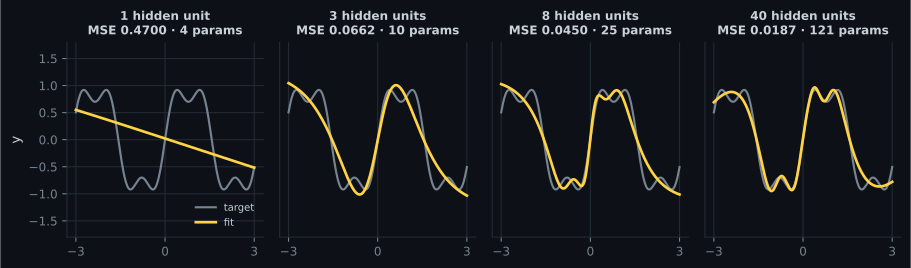
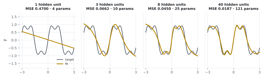
• The universal approximation theorem at 1, 3, 8 and 40 units — including how bad one unit is (MSE 0.4700).
• Width against depth at a fixed budget: 4×60 beat 1×128 with 42% fewer parameters, and 8×40 was worse than both.

The forward pass

An MLP with one hidden layer is three operations:

$$\mathbf{H} = \phi(\mathbf{X}\mathbf{W}_1 + \mathbf{b}_1), \qquad \hat{\mathbf{Y}} = \mathrm{softmax}(\mathbf{H}\mathbf{W}_2 + \mathbf{b}_2)$$

For a batch of $m$ rows with $n$ features, $h$ hidden units and $k$ classes, the shapes are forced:

Tensor	Shape
$\mathbf{X}$	$(m, n)$
$\mathbf{W}_1$	$(n, h)$
$\mathbf{b}_1$	$(h,)$ — broadcast across all $m$ rows
$\mathbf{H}$	$(m, h)$
$\mathbf{W}_2$	$(h, k)$
$\hat{\mathbf{Y}}$	$(m, k)$

diagram Diagram mermaid

  flowchart LR
  X["X: (m, 784)"] --> MM1["X @ W1
(784, 128)"]
  MM1 --> ADD1["+ b1
broadcast over m rows"]
  ADD1 --> ACT["relu"]
  ACT --> H["H: (m, 128)"]
  H --> MM2["H @ W2
(128, 10)"]
  MM2 --> ADD2["+ b2"]
  ADD2 --> SM["softmax over the 10 columns"]
  SM --> Y["Y: (m, 10)"]

Written in NumPy and compared against the Keras model holding the same weights:

forward_by_hand.py

hidden = np.maximum(x @ W1 + b1, 0.0)          # relu
logits = hidden @ W2 + b2
shifted = logits - logits.max(axis=1, keepdims=True)
probabilities = np.exp(shifted) / np.exp(shifted).sum(axis=1, keepdims=True)
 
print(probabilities)                  # [[0.570055 0.429945]]
print(model.predict(x, verbose=0))    # [[0.570055 0.429945]]

Maximum difference: $2.98 \times 10^{-8}$ — float32 rounding, nothing more. A Dense layer is a matmul, a broadcast add and an activation.

Counting parameters

Each layer contributes $(\text{inputs} \times \text{outputs})$ weights plus $\text{outputs}$ biases:

Architecture	Weights	Biases	Total
784-128-10	101,632	138	101,770
784-90-90-10	79,560	190	79,750
784-60-60-60-60-10	58,440	250	58,690
784-32-10	25,408	42	25,450

In 784-128-10, the first layer’s $784 \times 128 = 100{,}352$ weights are 98.6% of the whole model. Two consequences: the input dimension dominates a small MLP’s size, and adding hidden layers is far cheaper than widening the first one.

What a hidden layer actually does

The clearest test keeps the classifier fixed and changes only the representation. On the three-class spiral, with 450 training points:

Model	Test accuracy
logistic regression on the raw 2 features	0.6800
the MLP (32 hidden units, then softmax)	0.9600
logistic regression on the MLP’s 32 hidden units	0.9667

The third row is the point. It is the same algorithm as the first row, on the same labels, and it scores 0.2867 higher — because the hidden layer has re-expressed the two input coordinates as 32 features in which the classes are close to linearly separable.

A hidden layer is a learned change of coordinates. The final layer is still just a line; the hidden layers move the data until a line is enough. That is exactly what the hand-built XOR network did with OR and NAND, except learned rather than designed.

The universal approximation theorem, at four widths

The theorem says a network with one hidden layer and enough units can approximate any continuous function on a bounded interval to any accuracy. It does not say how many units, and it does not say training will find them. Fitting $y = \sin(2x) + 0.3\sin(6x)$ with one tanh layer:

figure One hidden layer, 600 epochs, widths 1 / 3 / 8 / 40 matplotlib

One tanh unit can only produce one S-shaped curve, so its best effort is a sloping line at MSE 0.4700. Three units find the primary wave. Forty capture the secondary wiggles at MSE 0.0187 — a 25x improvement for 121 parameters instead of 4.

Hidden units	Parameters	MSE
1	4	0.469952
3	10	0.066197
8	25	0.044981
40	121	0.018692

“Universal” is an existence claim, not a recipe. The gap between 1 and 3 units is a factor of 7 in MSE; between 8 and 40, a factor of 2.4. Capacity has diminishing returns, the same shape of curve that more training data produces.

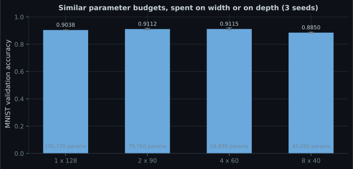
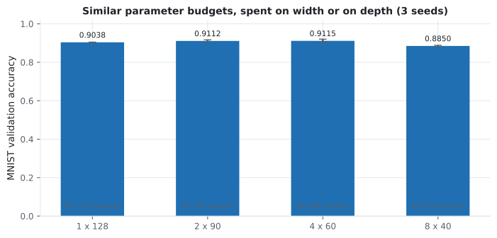
Width or depth?

If the theorem says one wide layer suffices, why go deep? Four architectures with comparable parameter budgets, MNIST, 8,000 rows, 6 epochs, three seeds each:

figure Similar budgets, spent on width or on depth matplotlib

The two middle configurations win while carrying fewer parameters — 4x60 matches 2x90 using 58,690 against 79,750, and beats the single wide layer's 101,770. At 8 layers of 40 units the accuracy drops to 0.8850: this plain MLP has no normalisation or residual connections, and depth without them stops paying.

Architecture	Parameters	Accuracy (mean of 3 seeds)
1 × 128	101,770	0.9038 (0.9015–0.9050)
2 × 90	79,750	0.9112 (0.9045–0.9170)
4 × 60	58,690	0.9115 (0.9035–0.9205)
8 × 40	43,290	0.8850 (0.8820–0.8885)

Read it carefully, because two of the readings cut against the usual slogans.

Depth is more parameter-efficient than width, up to a point. 4×60 reached 0.9115 with 42% fewer parameters than 1×128’s 0.9038. Layers compose features; width can only add more features at the same level of abstraction.

But “deeper is better” fails at 8 layers here. 0.8850 is worse than the single wide layer. Nothing is wrong with the code — a plain MLP with no batch normalisation, no residual connections and no learning-rate schedule runs into exactly the gradient problems measured on the activations page. Phase 2 is the toolkit that makes depth pay, and this row is the reason it exists.

The seed spread is not negligible. 4×60 ranged 0.9035–0.9205 across three seeds — a 0.0170 spread, which is larger than the gap between the top three architectures. Any comparison of “0.9112 vs 0.9115” without a spread attached is noise reporting.

The units you are paying for and not using

A ReLU unit whose pre-activation is negative for every input in the dataset outputs zero always. Its gradient is zero always too, so it can never recover. It is a parameter you store, multiply and never benefit from — and the count is not negligible:

figure MNIST, 8,000 rows, 8 epochs, 3 seeds, 64 units per layer matplotlib

Dead units grow with depth — 1.56% at one layer, 10.87% at eight — while accuracy stays inside 0.0077 across the whole range. The eight-layer network is carrying 512 units of which roughly 56 do nothing at all, for no gain over the one-layer network's 64. This is one concrete reason 'just add layers' stops paying long before the universal approximation theorem runs out of room.

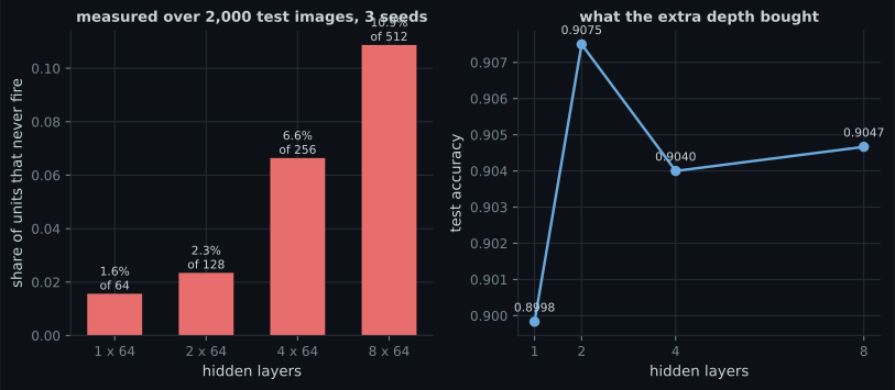
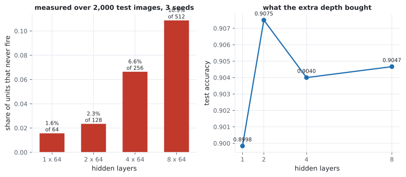
Hidden layers	Units	Dead share	Worst seed	Test accuracy
1 × 64	64	1.56%	3.12%	0.8998
2 × 64	128	2.34%	4.69%	0.9075
4 × 64	256	6.64%	8.59%	0.9040
8 × 64	512	10.87%	12.11%	0.9047

The accuracy column is the control. If depth were buying something, the dead-unit cost would be a trade; here it is 7× the waste for 0.0049 less accuracy than the two-layer model. Leaky ReLU, a smaller learning rate and better initialisation all reduce the count — but the first thing to do is measure it, because nothing in the training log mentions it.

Building one in Keras

mlp_keras.py

from tensorflow import keras
 
model = keras.Sequential([
    keras.layers.Input((784,)),
    keras.layers.Dense(128, activation="relu"),
    keras.layers.Dense(64, activation="relu"),
    keras.layers.Dense(10, activation="softmax"),
])
model.compile(optimizer="adam",
              loss="sparse_categorical_crossentropy",
              metrics=["accuracy"])
model.summary()

model.summary() prints the same arithmetic you did by hand:

Layer	Output shape	Parameters
dense	(None, 128)	100,480
dense_1	(None, 64)	8,256
dense_2	(None, 10)	650
total		109,386

None is the batch axis: pass 7 rows and you get (7, 10) out. Use sparse_categorical_crossentropy for integer labels and categorical_crossentropy for one-hot ones — mixing them up is the most common compile-time error in this phase.

See it move

sketch A tiny feed-forward network with weighted edges p5.js Pause Restart

Watch one forward pass ripple through the network: input signals travel to the hidden layer, ReLU fires, then the result travels on to the output.

The second sketch is the parameter budget. Move the sliders and watch where the parameters actually go — the first layer’s bar dwarfs everything else until the input dimension shrinks.

sketch Where the parameters go p5.js Pause Restart

Adjust the input dimension, hidden width and number of hidden layers, and see the parameter count per layer. The first layer dominates whenever the input is high-dimensional.

Pitfalls

Reading the universal approximation theorem as a recipe. It guarantees a width exists; it says nothing about how large, and nothing about whether gradient descent will find those weights. One unit’s best fit here was a sloping line at MSE 0.4700.

Assuming deeper is always better. 8×40 scored 0.8850 against 4×60’s 0.9115 on the same data. Plain MLPs stop benefiting from depth without the Phase 2 toolkit.

Comparing architectures on one seed. The 4×60 spread was 0.9035–0.9205. Differences smaller than that spread are not results.

Widening the first layer to add capacity. On a 784-input model, the first layer is already 98.6% of the parameters. An extra hidden layer is far cheaper than doubling that one.

Mismatching the loss to the label format. Integer labels need sparse_categorical_crossentropy; one-hot labels need categorical_crossentropy. The error message points at shapes, not at the loss.

Forgetting the activation between Dense layers. Two Dense layers with activation=None collapse into one, exactly as measured on the activations page — the parameters stay, the capacity does not.

Recap

• The forward pass is matmul, broadcast add, activation — verified against Keras to $2.98 \times 10^{-8}$.
• Parameters are $\text{inputs} \times \text{outputs} + \text{outputs}$ per layer, and the first layer is 98.6% of a 784-128-10 model.
• A hidden layer is a learned change of coordinates: the same logistic regression scored 0.6800 on raw features and 0.9667 on the MLP’s 32 hidden units.
• One hidden layer can approximate anything in principle; in practice 1 unit gave MSE 0.4700 and 40 units gave 0.0187 on the same curve.
• At matched budgets, 4×60 (0.9115, 58,690 params) beat 1×128 (0.9038, 101,770) — depth is more parameter-efficient — but 8×40 fell to 0.8850, which is what Phase 2 exists to fix.
• Seed spread on this task was up to 0.0170, larger than the gaps between the top three architectures.

pch.quizTag pch.quizDefaultTitle

1. A logistic regression scores 0.6800 on the spiral's two raw features and 0.9667 on the 32 hidden activations of a trained MLP. What does that demonstrate?

   A That logistic regression is a better classifier than an MLP B That the hidden layer's job is representation: it re-expresses the inputs in coordinates where a linear boundary is nearly sufficient — the classifier and the labels never changed C That 32 features are always better than 2 D That the MLP overfitted
   pch.quizShowAnswer

   B — That the hidden layer's job is representation: it re-expresses the inputs in coordinates where a linear boundary is nearly sufficient — the classifier and the labels never changed — The final layer of an MLP is still a linear model. Everything before it exists to move the data until a line is enough, which is exactly what the hand-built XOR network did with OR and NAND.

2. The universal approximation theorem says one hidden layer suffices. Why use more?

   A The theorem is wrong B It is an existence result with no bound on width and no guarantee that training finds the weights; measured here, 4x60 beat 1x128 while using 42% fewer parameters C Deeper networks always generalise better D One layer cannot represent non-linear functions
   pch.quizShowAnswer

   B — It is an existence result with no bound on width and no guarantee that training finds the weights; measured here, 4x60 beat 1x128 while using 42% fewer parameters — Depth composes features, so it often reaches the same accuracy with fewer parameters. But it is not unconditional: 8x40 scored 0.8850 against 4x60's 0.9115 on the same data.

3. In a 784-128-10 network, how much of the model is the first layer?

   A About a third B 98.6% — its 784 x 128 = 100,352 weights out of 101,770 parameters total, because the input dimension multiplies the first weight matrix C Half D It depends on the activation
   pch.quizShowAnswer

   B — 98.6% — its 784 x 128 = 100,352 weights out of 101,770 parameters total, because the input dimension multiplies the first weight matrix — This is why an extra hidden layer (width x width + width) is cheap while widening the first layer is expensive, and why convolutional layers exist for images.

4. You compare two architectures across 3 seeds: 0.9112 and 0.9115, with individual runs ranging 0.9045-0.9205. What can you conclude?

   A The second architecture is better B Nothing — the 0.0003 gap is far smaller than the 0.0170 seed spread, so the comparison needs more seeds or more data before it says anything C Both are overfitting D The difference is significant because the means differ
   pch.quizShowAnswer

   B — Nothing — the 0.0003 gap is far smaller than the 0.0170 seed spread, so the comparison needs more seeds or more data before it says anything — Reporting a mean without a spread is how architecture folklore gets created. Deep-learning results are draws from a distribution, and the spread here is larger than the effect.

5. You build Sequential([Dense(64), Dense(64), Dense(10, activation='softmax')]) with no activation on the hidden layers. What have you built?

   A A three-layer MLP B Effectively a single linear layer feeding a softmax — the two hidden weight matrices multiply into one, so the parameters remain but the capacity does not C A network that trains faster D An invalid model that will raise an error
   pch.quizShowAnswer

   B — Effectively a single linear layer feeding a softmax — the two hidden weight matrices multiply into one, so the parameters remain but the capacity does not — The collapse is measured on the activations page: two linear layers agree with one equivalent layer to 8.88e-16. The model runs, trains and quietly underperforms.

Next

You know what layers buy and what they cost. Continue to Activation Functions (ReLU, Sigmoid, Softmax) for the non-linearity that makes the stack more than one layer — then to Autograd from Scratch to build the gradient machinery these layers are trained with.

🧪 Try It Yourself

Exercise 1 – Count the parameters

pch.exerciseTag pch.exerciseTitle

Exercise 2 – Run the forward pass yourself

pch.exerciseTag pch.exerciseTitle

Exercise 3 – Match a parameter budget

pch.exerciseTag pch.exerciseTitle

Exercise 4 – One unit cannot fit a wave

pch.exerciseTag pch.exerciseTitle

Exercise 5 – Measure what the hidden layer buys

pch.exerciseTag pch.exerciseTitle

Exercise 6 – Trace the shapes

pch.exerciseTag pch.exerciseTitle