What you’ll learn

• Tom Mitchell’s T / E / P definition, and it plotted as a real curve: 0.4426 → 0.9722
• what “the model learns” means concretely — a number chosen to minimise an error
• why a baseline is the first thing you compute, not the last
• the vocabulary you will use for the rest of this module
• a measured demonstration that no algorithm can invent a signal that is not there

Intuition

Here is the whole idea, and it is genuinely this small.

You want a program that maps inputs to outputs — an image to a digit, an email to spam-or-not, a house to a price. You cannot write the rules, because you do not know them. What you do have is examples of the mapping: thousands of images with their correct digits.

So instead of writing the program, you write a program that searches for the program. You give it a family of candidate mappings, a way to score how badly a candidate does on your examples, and a procedure for finding a candidate that scores well.

That is machine learning. Three ingredients: a space of candidates, a measure of badness, and a search.

The definition

Tom Mitchell’s 1997 formulation is still the sharpest one available:

A computer program is said to learn from experience E with respect to some class of tasks T and performance measure P, if its performance at tasks in T, as measured by P, improves with experience E.

Its virtue is that all three letters are things you can point at:

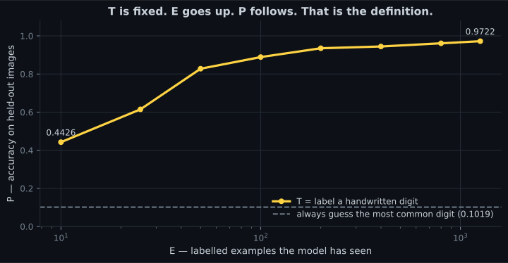
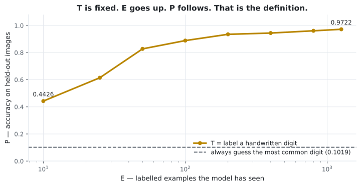
The definition is also testable, which is unusual for a definition. Fix T, fix P, vary E, and see whether P actually improves. Here it is, run for real:

figureMitchell's definition, measuredmatplotlib

Two details worth pausing on.

The baseline is 0.1019. Ten digits, roughly balanced, so guessing the most common one gets you about a tenth. Every accuracy number is only meaningful relative to that. A model at 0.85 on a problem whose baseline is 0.84 has learned essentially nothing.

The gains shrink. Going from 10 to 100 examples bought 0.4463. Going from 800 to 1,257 bought 0.0111. Almost every learning curve looks like this, and it is why “just get more data” stops being good advice at some point.

What “learning” actually is

Strip away the vocabulary and a model is a set of numbers, chosen to make an error as small as possible.

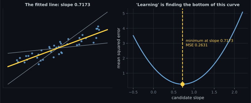
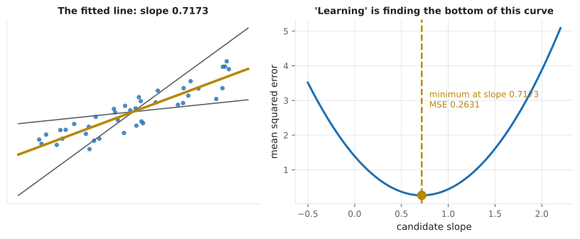
Take the simplest case: fit a straight line $y = wx + b$ to 40 points. The candidate space is every possible $(w, b)$. The measure of badness is the mean squared error:

Now the search. Hold $b$ fixed and sweep $w$:

There is exactly one bottom to that curve, and it sits at $w = 0.7173$. That number is the trained model. Everything else in this module — gradient descent, regularisation, boosting — is a more sophisticated way of finding the bottom of a more complicated curve.

figureFitting is finding the bottom of a curvematplotlib

See it move

There is nothing else in the box. A model family gives you the shape of the candidate line, a loss gives you the curve on the right, and training is the search for its lowest point.

ML is not magic

The most useful thing a beginner can internalise is what machine learning cannot do.

A model can only find relationships that are present in the features you give it. If the columns carry no information about the target, no algorithm recovers it. Not a bigger model, not more epochs, not a fashionable architecture.

Here is that claim, measured. Three thousand rows, a coin-flip target, and two feature sets: one where a column genuinely correlates with the label, one that is pure Gaussian noise. Same three algorithms on both:

figureThree algorithms, one dataset with nothing in itmatplotlib

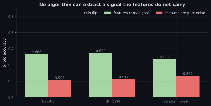
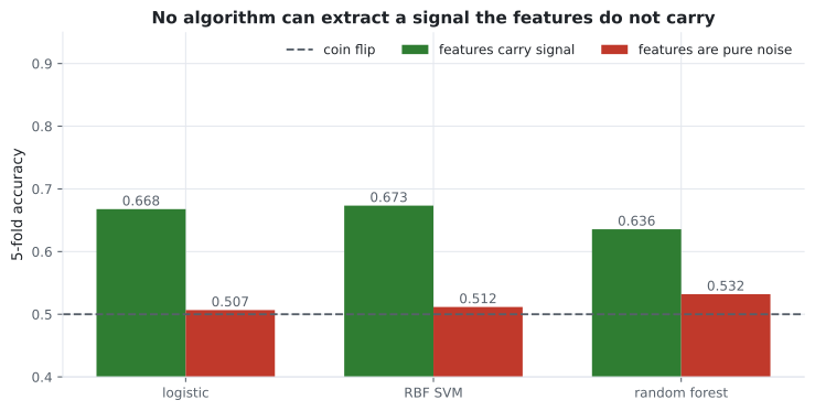
Note also the left-hand column: even with signal, the ceiling is 0.6733. The signal was deliberately weak, and no algorithm exceeded what the data allowed. The features set the ceiling. The algorithm decides how close you get to it. That ordering does not change anywhere in this module.

Core vocabulary

Every one of these terms appears in every later phase. Learn them once, here.

Two of these get confused constantly, so state the difference explicitly. Parameters are found by fitting — you never type them. Hyperparameters are set before fitting and control how the fitting happens. In LogisticRegression(C=0.1)LogisticRegression(C=0.1), CC is a hyperparameter; the coefficients it produces are parameters.

  flowchart LR
  H["Hyperparameters
you choose these"] --> F["Fitting procedure"]
  D["Training data
X and y"] --> F
  F --> P["Parameters
the procedure chooses these"]
  P --> M["Model"]
  M --> E["Evaluate on held-out data
THE only honest number"]

What ML is good for

The honest test is a checklist, and a problem should pass all four.

1. A pattern exists. There is a genuine relationship between inputs and output. Predicting a fair coin flip fails here, permanently.
2. You cannot write the rules. If you can specify the mapping precisely, write the code — it will be faster, cheaper, exactly correct and debuggable. Nobody should train a model to compute VAT.
3. You have data. Examples of the mapping, enough of them, representative of what production will look like.
4. Approximately right is useful. A model that is right 94% of the time has to be worth something. If only 100% will do, machine learning is the wrong tool.

In code

The whole loop, in fifteen lines:

from collections import Counter
 
from sklearn.datasets import load_digits
from sklearn.linear_model import LogisticRegression
from sklearn.model_selection import train_test_split
from sklearn.pipeline import make_pipeline
from sklearn.preprocessing import StandardScaler
 
X, y = load_digits(return_X_y=True)                  # E — the experience
X_train, X_test, y_train, y_test = train_test_split(
    X, y, test_size=0.3, random_state=0, stratify=y)
 
# The baseline FIRST. Always. Everything else is measured against it.
baseline = Counter(y_test).most_common(1)[0][1] / len(y_test)
print("baseline     ", round(baseline, 4))           # 0.1019
 
model = make_pipeline(StandardScaler(), LogisticRegression(max_iter=5000))
model.fit(X_train, y_train)                          # the search
 
print("train size   ", len(X_train))                 # 1257
print("test accuracy", round(model.score(X_test, y_test), 4))   # 0.9722

from collections import Counter
 
from sklearn.datasets import load_digits
from sklearn.linear_model import LogisticRegression
from sklearn.model_selection import train_test_split
from sklearn.pipeline import make_pipeline
from sklearn.preprocessing import StandardScaler
 
X, y = load_digits(return_X_y=True)                  # E — the experience
X_train, X_test, y_train, y_test = train_test_split(
    X, y, test_size=0.3, random_state=0, stratify=y)
 
# The baseline FIRST. Always. Everything else is measured against it.
baseline = Counter(y_test).most_common(1)[0][1] / len(y_test)
print("baseline     ", round(baseline, 4))           # 0.1019
 
model = make_pipeline(StandardScaler(), LogisticRegression(max_iter=5000))
model.fit(X_train, y_train)                          # the search
 
print("train size   ", len(X_train))                 # 1257
print("test accuracy", round(model.score(X_test, y_test), 4))   # 0.9722

Three habits worth forming from the very first model:

Split before you look. train_test_splittrain_test_split comes before any inspection, cleaning or plotting. Every decision you make after seeing the test set leaks information into your final number.

Compute the baseline first. It costs one line and it is the only thing that makes your accuracy interpretable.

Use a PipelinePipeline. Scaling belongs inside it. The moment preprocessing happens outside, it gets fitted on the test data too, and your score becomes fiction. Phase 2 covers why.

Pitfalls

Reporting accuracy with no baseline. 0.97 on digits is excellent (baseline 0.10). 0.97 on a problem with 97% negatives is worthless. The number alone tells you nothing.

Judging on the training set. Any sufficiently flexible model can memorise. Train accuracy is a measure of memory, not of learning.

Believing a bigger model fixes bad features. Measured above: the noise columns produced 0.5067, 0.5117 and 0.5320 across three very different algorithms. Feature quality is a ceiling.

Skipping the “can I just write the rule?” question. A great deal of production machine learning would have been three ifif statements.

Treating “the model is 94% accurate” as a property of the model. It is a property of the model on that test set. Change the population and the number changes.

Recap

• T / E / P: fix the task and the measure, add experience, and watch performance improve — measured here from 0.4426 to 0.9722 against a 0.1019 baseline.
• A model is a set of numbers minimising a loss. For a straight line that was slope 0.7173 with MSE 0.2631.
• The gains from more data shrink: +0.4463 from the first 90 examples, +0.0111 from the last 457.
• No algorithm can extract a signal the features do not carry — three of them landed within 0.032 of a coin flip on pure noise.
• Parameters are learned; hyperparameters are chosen.
• Split first, baseline first, pipeline always.

🧪 Try It Yourself

Exercise 1 – Baseline before model

Exercise 2 – Watch P improve with E

Exercise 3 – Find the bottom of the error curve

Exercise 4 – Prove that noise stays noise

Exercise 5 – Train accuracy is not learning

Exercise 6 – Price the next batch of data

Next

ML vs Traditional Programming — thirty hand-written rules against one fitted model on the same spam corpus, and the measurement that shows which of the two responds to more data.