
Boosting - Introduction to AdaBoost
What you’ll learn
Section titled “What you’ll learn”- boosting as the mirror image of bagging: sequential and aimed at bias, not variance
- the AdaBoost algorithm in five steps
- the predictor weight , derived and interpreted
- a complete round of AdaBoost computed by hand, weights and all
- why a learner at exactly 50% gets no vote, and one below 50% gets an inverted one
- why boosting is sensitive to noise where bagging is not
Intuition
Section titled “Intuition”Bagging trains many strong models independently and averages away their variance. Boosting does the opposite in every respect: it trains weak models one at a time, each one focused on the examples the previous ones got wrong, and attacks bias.
The mechanism is reweighting. After each round, misclassified examples get heavier and correctly classified ones get lighter. The next learner, fitted on those weights, is forced to pay attention to precisely the cases the committee currently fails on.
The remarkable claim — proved by Freund and Schapire in 1995 — is that any learner reliably better than chance can be boosted into an arbitrarily accurate one. A decision stump, a single split on a single feature, is enough.
  flowchart LR
  W1["equal weights"] --> S1["stump 1"]
  S1 --> E1["error → alpha 1"]
  E1 --> W2["reweight:
mistakes get heavier"]
  W2 --> S2["stump 2"]
  S2 --> E2["error → alpha 2"]
  E2 --> W3["reweight again"]
  W3 --> S3["stump m"]
  S1 --> V["weighted vote"]
  S2 --> V
  S3 --> V
Note the shape: every arrow is sequential. Stump 2 cannot start until stump 1’s errors are known, which is why boosting does not parallelise across members and a random forest does.
The math
Section titled “The math”The algorithm
Section titled “The algorithm”- Initialise every sample weight equally: .
- Fit a weak learner on the weighted data.
- Measure its weighted error rate:
- Weight the predictor:
- Reweight the samples, then renormalise so they sum to 1:
Repeat from step 2. The final prediction is the weighted vote:
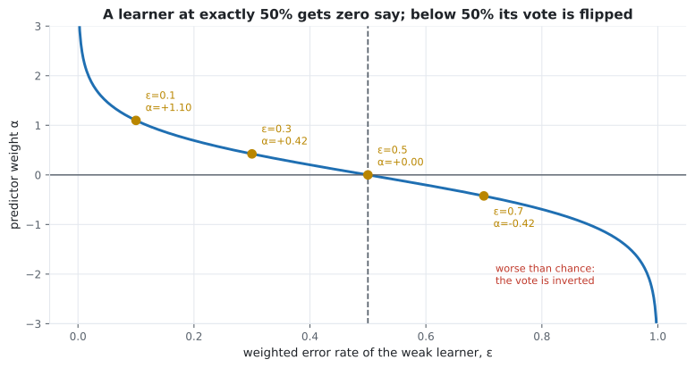
Reading the alpha formula
Section titled “Reading the alpha formula”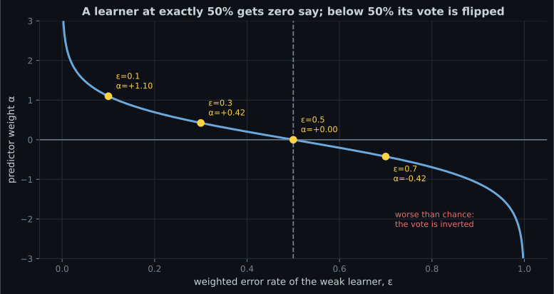
| Interpretation | ||
|---|---|---|
| 0.10 | +1.0986 | Strong learner, loud vote |
| 0.30 | +0.4236 | Useful |
| 0.40 | +0.2027 | Barely useful |
| 0.50 | 0.0000 | Coin flip — silenced entirely |
| 0.70 | −0.4236 | Reliably wrong, so its vote is flipped |
Three properties fall out of the logarithm:
- gives exactly zero. . A learner no better than chance contributes nothing, automatically — no special case in the code.
- The curve is antisymmetric about 0.5. A learner at 0.3 and one at 0.7 get weights of equal size and opposite sign. Being reliably wrong is exactly as useful as being reliably right, once you flip it.
- as . A perfect learner would dominate the vote — which is why AdaBoost stops early if a learner reaches zero error, and why weak learners are the point.
Worked example by hand
Section titled “Worked example by hand”Five samples, uniform initial weights of . Round 1’s stump misclassifies samples 2 and 4.
Step 1 — the weighted error.
Step 2 — the predictor weight.
Step 3 — the multipliers.
Step 4 — apply and renormalise.
| sample | correct? | before | multiplier | raw | after |
|---|---|---|---|---|---|
| 1 | ✓ | 0.2 | 0.8165 | 0.16330 | 0.16667 |
| 2 | ✗ | 0.2 | 1.2247 | 0.24495 | 0.25000 |
| 3 | ✓ | 0.2 | 0.8165 | 0.16330 | 0.16667 |
| 4 | ✗ | 0.2 | 1.2247 | 0.24495 | 0.25000 |
| 5 | ✓ | 0.2 | 0.8165 | 0.16330 | 0.16667 |
| 1.0 | 0.97980 | 1.0 |
Step 5 — read the result. The two misclassified samples went from 0.200 to 0.250, a 25% increase; the three correct ones fell to 0.1667. Their combined weight is now 0.50, up from 0.40 — the next stump faces a problem where half the mass is the cases the first stump could not handle.
Notice too that the mistakes’ total weight is now exactly . That is not a coincidence: the reweighting is constructed so the previous learner scores exactly 50% — and therefore — on the new distribution. Every round starts from a problem its predecessor finds impossible.
See it move
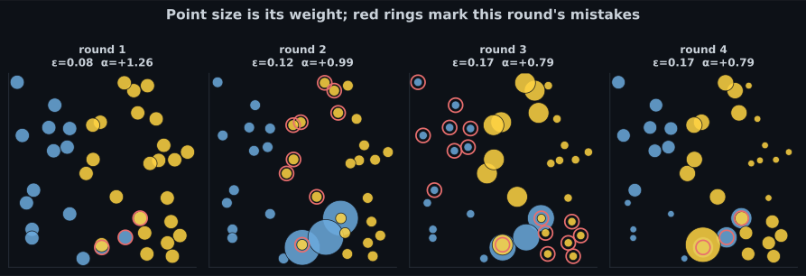
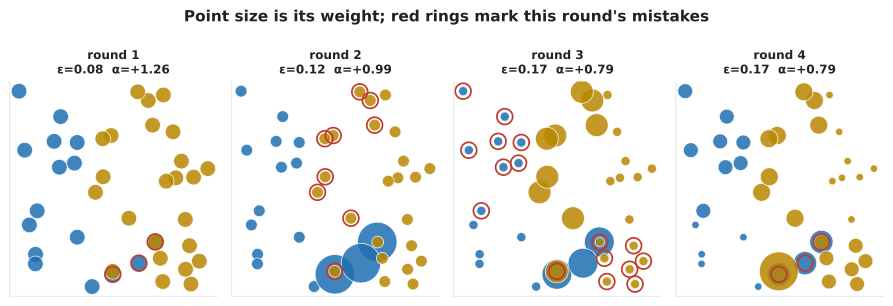
Section titled “See it move”The same loop, one round per beat. Watch the two mislabelled points in the middle swell until the stumps have no choice but to attend to them.
In code
Section titled “In code”from sklearn.datasets import load_breast_cancer
from sklearn.ensemble import AdaBoostClassifier
from sklearn.model_selection import cross_val_score
from sklearn.tree import DecisionTreeClassifier
X, y = load_breast_cancer(return_X_y=True)
for n_estimators in (1, 10, 50, 200):
model = AdaBoostClassifier(
DecisionTreeClassifier(max_depth=1), # a stump: one split, one feature
n_estimators=n_estimators,
learning_rate=1.0,
random_state=0,
)
print(f"{n_estimators:>3} stumps CV {cross_val_score(model, X, y, cv=5).mean():.4f}")
# 1 stumps CV 0.8998
# 10 stumps CV 0.9385
# 50 stumps CV 0.9666
# 200 stumps CV 0.9772One stump reaches 0.8998 — a single threshold on a single feature. Two hundred of them reach 0.9772, competitive with anything else in this curriculum on this dataset. That is the boosting claim, demonstrated: weak learners, chained, become strong.
Note the shape of the gains: 0.900 → 0.939 → 0.967 → 0.977. Each quadrupling of the budget buys roughly half the remaining error, which is the diminishing return you should expect.
Reading the weights back out
Section titled “Reading the weights back out”import numpy as np
model = AdaBoostClassifier(DecisionTreeClassifier(max_depth=1),
n_estimators=50, random_state=0).fit(X, y)
print("first five alphas:", model.estimator_weights_[:5].round(4))
print("first five errors:", model.estimator_errors_[:5].round(4))
# alpha should equal 0.5 * ln((1 - eps) / eps) for each stump
eps = model.estimator_errors_
manual = 0.5 * np.log((1 - eps) / eps)
print("formula matches:", np.allclose(manual, model.estimator_weights_ / 2, atol=1e-6))scikit-learn stores rather than (a harmless convention difference), which is worth knowing before you compare against the formula and conclude something is broken.
learning_rate: the second brake
Section titled “learning_rate: the second brake”The in step 4 scales every :
A smaller makes each learner contribute less, so more of them are needed — the same
shrinkage trade as in
gradient boosting.
learning_rate and n_estimators must be tuned together, and their product is roughly conserved.
Where boosting breaks
Section titled “Where boosting breaks”Bagging is robust to label noise: a mislabelled point ends up in about 63% of the bootstrap samples and gets outvoted. Boosting hunts it down.
A mislabelled example is misclassified every round by construction — no learner can get it right — so its weight grows exponentially. After enough rounds the ensemble is devoting most of its capacity to fitting a handful of corrupted labels.
| Data condition | Bagging | Boosting |
|---|---|---|
| Clean | Good | Usually better |
| Label noise | Robust | Degrades badly |
| Outliers in features | Robust | Sensitive |
| Class imbalance | Handles it with weights | Chases the minority, sometimes usefully |
pch.algoApi sklearn.ensemble.AdaBoostClassifier / AdaBoostRegressor
pch.algoAssumes
- Each weak learner is at least slightly better than chance on the weighted data
- The base learner supports sample weights
- Labels are reasonably clean — mislabelled points attract exponentially growing weight
pch.algoCost
- pch.algoTrain
O(m · n · estimators) — strictly sequential- pch.algoPredict
O(depth · estimators)- pch.algoMemory
O(estimators)
m = samples, n = features; the sequential dependency is why this cannot parallelise across estimators
pch.algoHyperparams
-
n_estimatorsdefault 50 Unlike a forest, this CAN overfit. Tune it, and pair it with learning_rate. -
learning_ratedefault 1.0 Scales every alpha. Lower needs more estimators; their product is roughly conserved. -
estimatordefault stump A depth-1 tree is the classic choice. Depth 2 or 3 captures interactions; deeper defeats the point. -
algorithmdefault SAMME SAMME.R used probabilities and converged faster; it is deprecated in recent versions in favour of SAMME.
pch.algoReachFor
- You want strong accuracy from very simple base learners
- The dataset is clean and modestly sized
- You want an ensemble with few hyperparameters to tune
- Interpretability of individual stumps has some value
pch.algoLookElsewhere
- Labels are noisy — the reweighting will chase the errors
- You need parallel training; boosting is inherently sequential
- The dataset is very large — consider histogram gradient boosting instead
- There are extreme outliers you cannot remove
Pitfalls
Section titled “Pitfalls”Compare
Section titled “Compare”| Bagging / Random Forest | AdaBoost | |
|---|---|---|
| Members | Strong, deep trees | Weak, stumps |
| Training | Parallel | Sequential |
| Attacks | Variance | Bias |
| Members weighted | Equally | By |
| More members overfit | No | Yes |
| Label noise | Robust | Fragile |
| Typical accuracy on clean tabular data | Very good | Often better |
-
A weak learner has a weighted error of exactly 0.5. What weight does AdaBoost give it?
alpha = 0.5 ln((1 - 0.5)/0.5) = 0.5 ln(1) = 0. A coin-flip learner is silenced automatically by the formula, with no special case needed.
pch.quizShowAnswer
C — Exactly 0 — alpha = 0.5 ln((1 - 0.5)/0.5) = 0.5 ln(1) = 0. A coin-flip learner is silenced automatically by the formula, with no special case needed.
-
A learner has a weighted error of 0.7. What does AdaBoost do with it?
The alpha curve is antisymmetric about 0.5. A learner wrong 70% of the time is right 70% of the time once you flip its output.
pch.quizShowAnswer
B — Gives it a negative weight of -0.4236, which inverts its vote — being reliably wrong is as useful as being reliably right — The alpha curve is antisymmetric about 0.5. A learner wrong 70% of the time is right 70% of the time once you flip its output.
-
After a round with error 0.4, what happens to the total weight of the misclassified samples?
The reweighting is constructed so each round hands its successor a problem the predecessor finds exactly as hard as guessing. That is what forces genuine specialisation.
pch.quizShowAnswer
B — It becomes exactly 0.5, so the previous learner would score 50% on the new distribution and earn zero weight — The reweighting is constructed so each round hands its successor a problem the predecessor finds exactly as hard as guessing. That is what forces genuine specialisation.
-
Why does AdaBoost degrade on noisy labels where bagging does not?
In bagging a bad point appears in 63% of samples and is outvoted. In boosting it is by definition always wrong, so the algorithm concludes it is the most important example.
pch.quizShowAnswer
B — A mislabelled point is misclassified every round, so its weight grows exponentially and the ensemble spends its capacity fitting corrupted labels — In bagging a bad point appears in 63% of samples and is outvoted. In boosting it is by definition always wrong, so the algorithm concludes it is the most important example.
🧪 Try It Yourself
Section titled “🧪 Try It Yourself”Exercise 1 – The alpha formula
Section titled “Exercise 1 – The alpha formula”Exercise 2 – One round of reweighting
Section titled “Exercise 2 – One round of reweighting”Exercise 3 – Weak learners become strong
Section titled “Exercise 3 – Weak learners become strong”Exercise 4 – A weighted majority vote
Section titled “Exercise 4 – A weighted majority vote”Exercise 5 – Watch boosting chase a bad label
Section titled “Exercise 5 – Watch boosting chase a bad label”- Boosting is bagging’s mirror image: weak learners, trained sequentially, attacking bias.
- gives +1.099 at 10% error, exactly 0 at 50%, and −0.424 at 70% — the vote is inverted rather than discarded.
- Hand-worked round: error 0.4, , mistake weights rise from 0.200 to 0.250 and their total mass becomes exactly 0.5.
- Each round hands its successor a problem the previous learner finds no better than chance.
- One decision stump on breast cancer scores 0.8998; two hundred score 0.9772.
n_estimatorscan overfit here, unlike a random forest, andlearning_ratetrades against it.- Boosting is fragile to label noise for exactly the reason it is powerful on clean data.
Exercise 6 – Run one AdaBoost weight update by hand
Section titled “Exercise 6 – Run one AdaBoost weight update by hand”Continue to Gradient Boosting (XGBoost, LightGBM, CatBoost) — the same sequential idea with reweighting replaced by gradient descent in function space, and the family of libraries that dominates tabular machine learning.
pch.coffeeTagline
pch.coffeeCtapch.feedbackHeading
pch.feedbackSubheading