Matrix Phylogeny

Seven pages have introduced classes of matrices — invertible, defective, normal, symmetric, positive definite, orthogonal, diagonal — and a decomposition for most of them. This page is the map.

The word phylogenetic describes how we capture the relationships among individuals or groups, and comes from the Greek words for “tribe” and “source”. A phylogenetic tree of matrices is exactly what Figure 4.13 draws: black arrows for is a subset of, blue labels for what you can do with it.

What you’ll learn

• The whole tree: which matrix classes contain which, in the order the book presents them.
• Which decomposition attaches to each class, and what condition unlocks it.
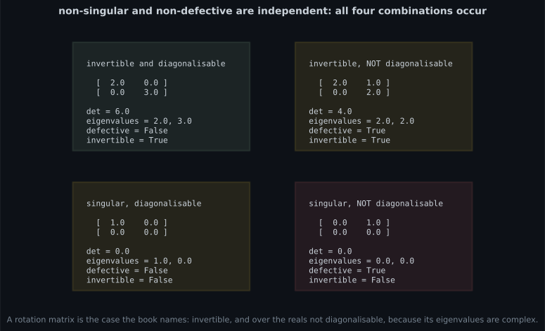
• Why non-singular and non-defective are independent — the book’s own caveat, with a witness in each of the four quadrants.
• What normal means ($\mathbf{A}^\top\mathbf{A} = \mathbf{A}\mathbf{A}^\top$) and why it sits between non-defective and symmetric.
• A measured census: how often each construction of random matrix actually lands in each class.
• Which class np.linalg.qr puts you in, which is not the one most people assume.

Intuition: two independent questions, then a chain of restrictions

The tree looks complicated because it answers two different questions at the same level.

The first is can you invert it? — decided by the determinant. The second is can you diagonalise it? — decided by whether there are $n$ independent eigenvectors. These are independent: a matrix can be either, both or neither. The book says so explicitly, and it is the most commonly mis-remembered fact in the chapter.

Below the non-defective branch, though, everything is a chain of tightening restrictions, and each tightening buys something:

$$\text{non-defective} \supset \text{normal} \supset \text{symmetric} \supset \text{positive definite} \supset \text{diagonal (positive)} \supset \{\mathbf{I}\}$$

with orthogonal hanging off normal in a different direction.

diagram Diagram mermaid

  flowchart TD
  R["Real matrices A ∈ ℝⁿˣᵐ
∃ pseudo-inverse, ∃ SVD"]
  R --> NS["Non-square, n ≠ m
ℝⁿˣᵐ"]
  R --> SQ["Square, ℝⁿˣⁿ
∃ determinant, ∃ trace"]
  SQ -->|"det ≠ 0"| REG["Regular / invertible
∃ inverse matrix"]
  SQ -->|"det = 0"| SING1["Singular"]
  SQ -->|"basis of eigenvectors"| ND["Non-defective
(diagonalizable)
∃ eigendecomposition"]
  SQ -->|"no basis of eigenvectors"| DEF["Defective"]
  ND -->|"AᵀA = AAᵀ"| NORM["Normal"]
  ND -->|"AᵀA ≠ AAᵀ"| NONNORM["Non-normal"]
  NORM -->|"AᵀA = AAᵀ = I"| ORTH["Orthogonal
Aᵀ = A⁻¹
columns are orthonormal"]
  ORTH --> ROT["Rotation
det = +1"]
  ORTH -->|"det ≠ 0"| REG
  NORM --> SYM["Symmetric, S = Sᵀ
eigenvalues ∈ ℝ"]
  SYM --> PD["Positive definite
xᵀPx > 0
∃ Cholesky
eigenvalues > 0"]
  PD -->|"det ≠ 0"| REG
  SYM --> DIAG["Diagonal D"]
  DIAG --> ID["Identity matrix I"]

That is the book’s Figure 4.13, with the blue operations folded into the boxes.

The math

The trunk: every real matrix

For all real matrices $\mathbf{A} \in \mathbb{R}^{n\times m}$, the pseudo-inverse and the SVD exist. That is the widest statement in the chapter, and it is why §4.5 came last: it needs no hypothesis at all.

For non-square matrices ($n \neq m$) that is where the tree stops. There is no determinant, no trace, no eigenvalue — those all require a square matrix, since $\mathbf{A}\mathbf{x} = \lambda\mathbf{x}$ needs $\mathbf{A}\mathbf{x}$ to live in the same space as $\mathbf{x}$.

The first fork: invertibility

Focusing on square matrices $\mathbf{A} \in \mathbb{R}^{n\times n}$, the determinant informs us whether the matrix possesses an inverse — that is, whether it belongs to the class of regular, invertible matrices. This is §4.1’s Theorem 4.1: $\det\mathbf{A} \neq 0$ if and only if $\mathbf{A}^{-1}$ exists.

The second fork: diagonalisability

If the square $n\times n$ matrix possesses $n$ linearly independent eigenvectors, then the matrix is non-defective and an eigendecomposition exists (§4.4’s Theorem 4.20; the sufficient condition of distinct eigenvalues is Theorem 4.12). Repeated eigenvalues may result in defective matrices, which cannot be diagonalized.

Non-singular and non-defective are not the same

This is the book’s own warning and it deserves the emphasis. Its example: a rotation matrix will be invertible — its determinant is nonzero, in fact $+1$ — but not diagonalizable in the real numbers, because its eigenvalues are not guaranteed to be real.

All four combinations occur, and there is a small witness for each:

	invertible	singular
diagonalisable	$\begin{bmatrix}2&0\\0&3\end{bmatrix}$, $\det = 6$	$\begin{bmatrix}1&0\\0&0\end{bmatrix}$, $\det = 0$, eigenvalues $1, 0$
not diagonalisable	$\begin{bmatrix}2&1\\0&2\end{bmatrix}$, $\det = 4$, $\lambda = 2$ twice with one eigenvector	$\begin{bmatrix}0&1\\0&0\end{bmatrix}$, $\det = 0$, $\lambda = 0$ twice with one eigenvector

Neither property implies the other in either direction.

Down the non-defective branch: normal

Normal matrices

$\mathbf{A}$ is normal if

$$\mathbf{A}^\top\mathbf{A} = \mathbf{A}\mathbf{A}^\top$$

This is the condition that makes the two Gram matrices of §4.5 coincide — and therefore makes the left- and right-singular vectors the same, which is exactly why normal matrices are the ones whose SVD and eigendecomposition line up. Over the reals, normal is the natural home of “diagonalisable by an orthogonal change of basis”.

If the more restrictive condition holds that

$$\mathbf{A}^\top\mathbf{A} = \mathbf{A}\mathbf{A}^\top = \mathbf{I}$$

then $\mathbf{A}$ is orthogonal (Definition 3.8). The set of orthogonal matrices is a subset of the regular matrices and satisfies $\mathbf{A}^\top = \mathbf{A}^{-1}$ — the cheapest inverse in linear algebra. Orthogonal matrices with $\det = +1$ are rotations; with $\det = -1$ they are reflections.

Symmetric, and below

Normal matrices have a frequently encountered subset, the symmetric matrices $\mathbf{S} \in \mathbb{R}^{n\times n}$ satisfying $\mathbf{S} = \mathbf{S}^\top$. Symmetric matrices have only real eigenvalues — the spectral theorem, 4.15, which the chapter has leaned on repeatedly.

A subset of the symmetric matrices consists of the positive definite matrices $\mathbf{P}$ satisfying

$$\mathbf{x}^\top\mathbf{P}\mathbf{x} > 0 \quad \text{for all } \mathbf{x} \in \mathbb{R}^n\setminus\{\mathbf{0}\}$$

In this case a unique Cholesky decomposition exists (Theorem 4.18). Positive definite matrices have only positive eigenvalues and are always invertible — a nonzero determinant follows, since the determinant is the product of the eigenvalues.

Another subset of the symmetric matrices consists of the diagonal matrices $\mathbf{D}$. Diagonal matrices are closed under multiplication and addition, but do not necessarily form a group — that is only the case if all diagonal entries are nonzero, so that the matrix is invertible. A special diagonal matrix is the identity $\mathbf{I}$.

From the book

Section 4.7 and Figure 4.13. The etymology of “phylogenetic” is the book’s own margin note. Black arrows in Figure 4.13 mean “is a subset of” and blue labels are the available operations. The section states in order: the SVD and pseudo-inverse exist for all real matrices; the determinant decides invertibility for square ones; $n$ independent eigenvectors make a matrix non-defective and give an eigendecomposition (Theorem 4.12); non-singular and non-defective are not the same, with a rotation matrix as the counterexample; normal means $\mathbf{A}^\top\mathbf{A} = \mathbf{A}\mathbf{A}^\top$; orthogonal is the stricter $\mathbf{A}^\top\mathbf{A} = \mathbf{A}\mathbf{A}^\top = \mathbf{I}$ with $\mathbf{A}^\top = \mathbf{A}^{-1}$ (Definition 3.8); symmetric matrices are a subset of normal ones and have real eigenvalues; positive definite matrices are a subset of symmetric ones with a unique Cholesky (Theorem 4.18), positive eigenvalues and nonzero determinant; diagonal matrices are a subset of symmetric ones, closed under multiplication and addition but a group only when every diagonal entry is nonzero; and the identity is a special diagonal matrix.

Worked example by hand

Every class, on one matrix each

matrix	invertible	non-defective	normal	symmetric	pos. def.	orthogonal	diagonal
$\begin{bmatrix}0&1\\0&0\end{bmatrix}$	no	no	no	no	no	no	no
$\begin{bmatrix}2&1\\0&2\end{bmatrix}$	yes	no	no	no	no	no	no
$\begin{bmatrix}4&2\\1&3\end{bmatrix}$	yes	yes	no	no	no	no	no
$\begin{bmatrix}0&-1\\1&0\end{bmatrix}$	yes	yes over $\mathbb{C}$, no over $\mathbb{R}$	yes	no	no	yes	no
$\begin{bmatrix}2&1\\1&2\end{bmatrix}$	yes	yes	yes	yes	yes	no	no
$\begin{bmatrix}2&1\\1&-2\end{bmatrix}$	yes	yes	yes	yes	no	no	no
$\begin{bmatrix}3&0\\0&2\end{bmatrix}$	yes	yes	yes	yes	yes	no	yes
$\begin{bmatrix}1&0\\0&1\end{bmatrix}$	yes	yes	yes	yes	yes	yes	yes

Two rows repay attention.

Row 4, the $90°$ rotation $\begin{bmatrix}0&-1\\1&0\end{bmatrix}$, is normal and orthogonal, with eigenvalues $\pm i$. So “normal” does not imply “real eigenvalues” — only symmetric does. Over $\mathbb{C}$ it has two distinct eigenvalues and two independent eigenvectors, so it is perfectly diagonalisable there; over $\mathbb{R}$ there is no eigenvector at all. This is why the book’s caveat says “not diagonalizable in the real numbers”, and why the entry in that column needs a field, not just a yes or no. A numerical classifier built on np.linalg.eigvals, which returns complex arrays, will report it as non-defective — correctly, over $\mathbb{C}$.

Row 6, $\begin{bmatrix}2&1\\1&-2\end{bmatrix}$, is symmetric with eigenvalues $\pm\sqrt5 \approx \pm2.236$ — real, as the spectral theorem demands, but one is negative, so it is not positive definite and has no Cholesky. Symmetry gets you real eigenvalues; positive definiteness is a further condition.

Verified

phylogeny.py

import numpy as np
 
TOL = 1e-8
 
def is_defective(M, tol=1e-7):
    n = M.shape[0]
    seen, total = [], 0
    for lam in np.linalg.eigvals(M):
        if any(abs(lam - u) < 1e-6 for u in seen):
            continue
        seen.append(lam)
        s = np.linalg.svd(M - lam * np.eye(n), compute_uv=False)
        total += int(np.sum(s < tol * max(1.0, float(s[0]))))
    return total < n
 
def classify(M):
    n = M.shape[0]
    sym = bool(np.allclose(M, M.T, atol=TOL))
    posdef = False
    if sym:
        try:
            np.linalg.cholesky(M)
            posdef = True
        except np.linalg.LinAlgError:
            posdef = False
    return {
        "invertible":  abs(float(np.linalg.det(M))) > TOL,
        "non-defect":  not is_defective(M),
        "normal":      bool(np.allclose(M.T @ M, M @ M.T, atol=TOL)),
        "symmetric":   sym,
        "pos.def":     posdef,
        "orthogonal":  bool(np.allclose(M.T @ M, np.eye(n), atol=TOL)),
        "diagonal":    bool(np.allclose(M, np.diag(np.diag(M)), atol=TOL)),
    }
 
cases = {
    "nilpotent  [[0,1],[0,0]]": [[0.0, 1], [0, 0]],
    "Jordan     [[2,1],[0,2]]": [[2.0, 1], [0, 2]],
    "generic    [[4,2],[1,3]]": [[4.0, 2], [1, 3]],
    "rotation   [[0,-1],[1,0]]": [[0.0, -1], [1, 0]],
    "SPD        [[2,1],[1,2]]": [[2.0, 1], [1, 2]],
    "indefinite [[2,1],[1,-2]]": [[2.0, 1], [1, -2]],
    "diagonal   [[3,0],[0,2]]": [[3.0, 0], [0, 2]],
    "identity   [[1,0],[0,1]]": [[1.0, 0], [0, 1]],
}
 
keys = list(classify(np.eye(2)).keys())
print(f"{'matrix':26}" + "".join(f"{k:>12}" for k in keys) + f"{'eigenvalues':>26}")
for name, M in cases.items():
    M = np.asarray(M, dtype=float)
    c = classify(M)
    ev = np.linalg.eigvals(M)
    evs = ", ".join(f"{v.real:+.3f}{v.imag:+.3f}j" if abs(v.imag) > 1e-12 else f"{v.real:+.3f}"
                    for v in ev)
    print(f"{name:26}" + "".join(f"{('yes' if c[k] else 'no'):>12}" for k in keys) + f"{evs:>26}")

output

matrix                      invertible  non-defect      normal   symmetric     pos.def  orthogonal    diagonal               eigenvalues
nilpotent  [[0,1],[0,0]]            no          no          no          no          no          no          no            +0.000, +0.000
Jordan     [[2,1],[0,2]]           yes          no          no          no          no          no          no            +2.000, +2.000
generic    [[4,2],[1,3]]           yes         yes          no          no          no          no          no            +5.000, +2.000
rotation   [[0,-1],[1,0]]          yes         yes         yes          no          no         yes          no+0.000+1.000j, +0.000-1.000j
SPD        [[2,1],[1,2]]           yes         yes         yes         yes         yes          no          no            +3.000, +1.000
indefinite [[2,1],[1,-2]]          yes         yes         yes         yes          no          no          no            +2.236, -2.236
diagonal   [[3,0],[0,2]]           yes         yes         yes         yes         yes          no         yes            +3.000, +2.000
identity   [[1,0],[0,1]]           yes         yes         yes         yes         yes         yes         yes            +1.000, +1.000

Read down the columns and the tree appears. Every yes in pos.def has a yes in symmetric to its left, which has a yes in normal, which has a yes in non-defect. The containments hold in every row, which is what a tree of subsets should look like.

Two rows show where the tree branches rather than nests. The Jordan row is invertible yes with non-defect no — the book’s caveat, and note that nothing to its right is yes either, because a defective matrix cannot be normal. The rotation row is normal yes with symmetric no, and its eigenvalue column is the only complex one: $\pm i$. That is the pair to remember — normal buys you an orthogonal diagonalisation, but only symmetry buys you real eigenvalues.

Notice also that this classifier reports the rotation as non-defect yes, because np.linalg.eigvals works over $\mathbb{C}$ and finds two distinct eigenvalues with two independent eigenvectors there. That is the right answer to the question the code asks. It is not the answer to the question the book asks, which is about $\mathbb{R}$ — and the discrepancy is a reminder that “diagonalisable” is incomplete without a field.

See it move

sketch Where does this matrix sit in the tree? p5.js Pause Restart

Edit a 2x2 matrix with the four knobs, or press a preset. Every class in the phylogeny lights up or stays dark, the eigenvalues are shown (complex when they are), and the tree redraws with the matrix's path highlighted. Watch what breaks first as you move away from the identity.

sketch Which classes are common, and which need arranging? p5.js Pause Restart

Each column is a matrix class; each row is a way of generating a random 3x3 matrix. Press sample to draw more and watch the percentages settle. The point is which cells stay at zero: no amount of sampling makes a Gaussian matrix symmetric, because symmetry is a measure-zero coincidence.

matrixThe rotation matrix: invertible, and not diagonalizable over the realslinear map on R^2

0-110

columns of A = images of e1, e2

det A 1area factor 1orientation preserved

1e1, e2 = (1, 0), (0, 1)          # the basis we start from2A @ e1  ==  A[:, 0]              # first column IS the image of e13A @ e2  ==  A[:, 1]              # second column IS the image of e24# linearity: A(x1 e1 + x2 e2) = x1 (A e1) + x2 (A e2)5det(A) = a*d - b*c               # signed area of the image of the unit square6A @ v = lam * v                  # an eigenvector keeps its direction

det A1A e1(0, 1)A e2(-1, 0)

basisThe plane before anything happens, with the standard basis e1 = (1, 0) and e2 = (0, 1) and the unit square they span.

Play‹›1/7⟲

Determinant +1, so certainly invertible. But its characteristic polynomial is lambda squared plus one, whose roots are plus and minus i — so there is no real eigenvector and no real eigendecomposition. This is the book's own counterexample to the idea that non-singular and non-defective are the same.

From scratch

phylogeny_census.py

import numpy as np
 
TOL = 1e-8
PROPS = ["invertible", "non-defective", "normal", "symmetric",
         "pos. definite", "orthogonal", "diagonal", "rotation"]
 
def is_defective(M, tol=1e-7):
    n = M.shape[0]
    seen, total = [], 0
    for lam in np.linalg.eigvals(M):
        if any(abs(lam - u) < 1e-6 for u in seen):
            continue
        seen.append(lam)
        s = np.linalg.svd(M - lam * np.eye(n), compute_uv=False)
        total += int(np.sum(s < tol * max(1.0, float(s[0]))))
    return total < n
 
def classify(M):
    n = M.shape[0]
    sym = bool(np.allclose(M, M.T, atol=TOL))
    posdef = False
    if sym:
        try:
            np.linalg.cholesky(M)
            posdef = True
        except np.linalg.LinAlgError:
            posdef = False
    orth = bool(np.allclose(M.T @ M, np.eye(n), atol=TOL))
    return {
        "invertible": abs(float(np.linalg.det(M))) > TOL,
        "non-defective": not is_defective(M),
        "normal": bool(np.allclose(M.T @ M, M @ M.T, atol=TOL)),
        "symmetric": sym,
        "pos. definite": posdef,
        "orthogonal": orth,
        "diagonal": bool(np.allclose(M, np.diag(np.diag(M)), atol=TOL)),
        "rotation": orth and float(np.linalg.det(M)) > 0,
    }
 
rng = np.random.default_rng(41)
n = 3
 
def jordan():
    J = np.eye(n); J[0, 1] = 1.0
    S = rng.normal(size=(n, n))
    while abs(np.linalg.det(S)) < 0.3:
        S = rng.normal(size=(n, n))
    return S @ J @ np.linalg.inv(S)
 
families = [
    ("Gaussian",      lambda: rng.normal(size=(n, n))),
    ("small integer", lambda: rng.integers(-2, 3, size=(n, n)).astype(float)),
    ("symmetric",     lambda: (lambda M: M + M.T)(rng.normal(size=(n, n)))),
    ("SPD",           lambda: (lambda M: M @ M.T + n * np.eye(n))(rng.normal(size=(n, n)))),
    ("orthogonal",    lambda: np.linalg.qr(rng.normal(size=(n, n)))[0]),
    ("diagonal",      lambda: np.diag(rng.normal(size=n))),
    ("Jordan-like",   jordan),
]
 
trials = 1200
print(f"{'construction':>15}" + "".join(f"{p[:13]:>15}" for p in PROPS))
for name, make in families:
    hits = np.zeros(len(PROPS))
    for _ in range(trials):
        c = classify(make())
        hits += np.array([1.0 if c[p] else 0.0 for p in PROPS])
    pct = 100.0 * hits / trials
    print(f"{name:>15}" + "".join(f"{v:>15.2f}" for v in pct))

output

   construction     invertible  non-defective         normal      symmetric  pos. definite     orthogonal       diagonal       rotation
       Gaussian         100.00         100.00           0.00           0.00           0.00           0.00           0.00           0.00
  small integer          83.83          94.33           0.67           0.58           0.00           0.00           0.00           0.00
      symmetric         100.00         100.00         100.00         100.00           2.50           0.00           0.00           0.00
            SPD         100.00         100.00         100.00         100.00         100.00           0.00           0.00           0.00
     orthogonal         100.00         100.00         100.00           0.00           0.00         100.00           0.00         100.00
       diagonal         100.00         100.00         100.00         100.00          12.67           0.00         100.00           0.00
    Jordan-like         100.00           0.00           0.00           0.00           0.00           0.00           0.00           0.00

Six readings, in order of how surprising they are.

The Jordan-like row is the book’s counterexample, sampled. $100\%$ invertible, $0\%$ non-defective. The two properties do not merely fail to imply each other in principle; you can generate a thousand matrices that split them.

The diagonal row’s $12.67\%$ positive definite is a coin-flip check. A diagonal matrix with three independent standard-normal entries is positive definite exactly when all three are positive, which has probability $1/8 = 12.5\%$. Measuring $12.67\%$ over $1200$ draws confirms the classifier is testing what it claims to.

The symmetric row is only $2.50\%$ positive definite. Symmetry gets you real eigenvalues, not positive ones. $\mathbf{M} + \mathbf{M}^\top$ for Gaussian $\mathbf{M}$ has eigenvalues spread either side of zero, and needing all three positive is rare. The book’s chain symmetric $\supset$ positive definite is a strict containment, and this is how strict.

The Gaussian row has zeros in five of eight columns, and they will never fill in. Symmetry requires $a_{ij} = a_{ji}$ exactly, an equality between two independent continuous random variables — probability zero. All the structured classes are measure-zero coincidences, which is why every one of them has to be constructed.

Small-integer matrices are only $83.83\%$ invertible. Over a range of five integers, $\det = 0$ happens. And $94.33\%$ non-defective — repeats become possible once entries are discrete, exactly as §4.4’s census found.

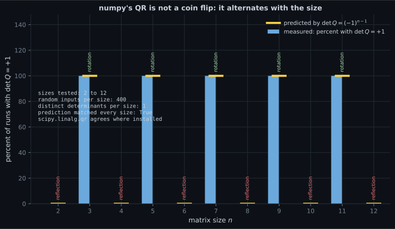
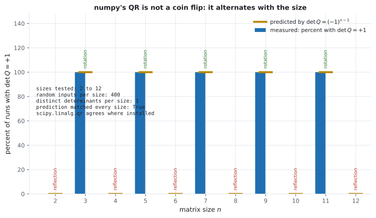
The orthogonal row is $100\%$ rotation, and that is an artefact of $n = 3$. np.linalg.qr returns a $\mathbf{Q}$ with $\det\mathbf{Q} = (-1)^{n-1}$, which is $+1$ for $n = 3$. In any even dimension the same code returns reflections, every time. The last figure on this page measures it.

On real data

figure The tree, sampled matplotlib

1200 random 3x3 matrices per construction. The zeros are the message: a Gaussian matrix is never symmetric, normal, orthogonal or diagonal, because each is an exact equality between continuous quantities. The Jordan-like row is 100% invertible and 0% non-defective.

figure Which class implies which, measured matplotlib

Every cell is the share of sampled matrices with the row property that also have the column property. The 100% cells reproduce the tree's containments — symmetric implies normal, positive definite implies symmetric. The two cells that matter are invertible-implies-non-defective at 85.0% and non-defective-implies-invertible at 98.0%: neither is 100%.

figure All four combinations occur matplotlib

A witness in each quadrant: diag(2,3) is invertible and diagonalisable, [[2,1],[0,2]] is invertible and defective, diag(1,0) is singular and diagonalisable, and [[0,1],[0,0]] is both singular and defective. The book's own example, a rotation matrix, is the second quadrant with complex eigenvalues instead of a repeat.

figure Which class does np.linalg.qr put you in? matplotlib

400 random inputs at each size from 2 to 12. The determinant of Q is (-1) to the (n-1), exactly, with no exceptions in 4400 trials: minus one for even n, plus one for odd. Householder QR applies n-1 reflections and each has determinant minus one. So in every even dimension numpy hands back a reflection, never a rotation.

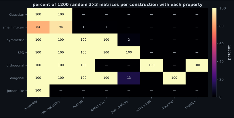
Reading the plot

From the census heatmap. Read the zeros, not the hundreds. Five of the eight columns are empty in the Gaussian row, and no amount of sampling changes that — symmetry, normality, orthogonality and diagonality are all exact equalities between continuous quantities, so their probability is zero. Every interesting class in this chapter has to be built, and that is why the book’s tree is a tree of constructions rather than a partition of the typical case.

The two rows that are not zero-or-one are the informative ones: small integer at $83.83\%$ invertible and $94.33\%$ non-defective, and diagonal at $12.67\%$ positive definite. The last one is a check on the classifier, since the theoretical value is $12.5\%$.

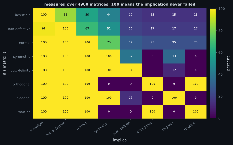
From the implications heatmap. The $100\%$ cells are the tree’s black arrows, recovered from data: symmetric $\Rightarrow$ normal, positive definite $\Rightarrow$ symmetric $\Rightarrow$ normal $\Rightarrow$ non-defective, orthogonal $\Rightarrow$ normal, diagonal $\Rightarrow$ symmetric. None of those needed to be told to the sampler; they fall out.

The cells that are not $100\%$ are where the tree branches rather than nests:

given	also has	share
invertible	non-defective	$85.0\%$
non-defective	invertible	$98.0\%$
normal	symmetric	$75.0\%$
symmetric	positive definite	$38.8\%$
symmetric	orthogonal	$0.0\%$
orthogonal	symmetric	$0.0\%$

The first two rows are the book’s caveat as a pair of numbers: neither direction is an implication. The last two are worth noticing too — in this sample no orthogonal matrix was symmetric and vice versa. That is not a theorem (the identity and any reflection matrix are both) but it reflects that the two branches leave normal in different directions, so a matrix in both is a further coincidence.

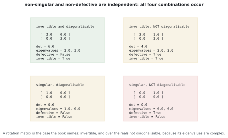
From the four-quadrant figure. Read the defective and invertible lines in each box. All four $(\text{yes},\text{no})$ pairs appear, which is the definition of independent. The book names the rotation matrix as its example and puts it in the top-right quadrant; the figure uses $\begin{bmatrix}2&1\\0&2\end{bmatrix}$ there instead, because a repeated real eigenvalue makes the failure visible without leaving the reals. Both work; the rotation’s failure is complex eigenvalues, the Jordan block’s is a deficient eigenspace.

From the QR figure. This is the practical one, and it corrects a widespread assumption. Ask for a random orthogonal matrix with np.linalg.qr(np.random.normal(size=(n,n)))[0] and you do not get a uniformly random element of the orthogonal group — you get one whose determinant is $(-1)^{n-1}$, deterministically. Over $4400$ trials across eleven sizes there was not one exception.

The reason is the algorithm: Householder QR builds $\mathbf{Q}$ from $n-1$ reflections, and each reflection has determinant $-1$, so $\det\mathbf{Q} = (-1)^{n-1}$. For $n=3$ that is $+1$, which is why the census row said $100\%$ rotation — a fact about three dimensions, not about QR. In $n = 2, 4, 6, \dots$ the same call returns a reflection every time. If you need a rotation, negate a column when the determinant is negative.

Pitfalls

Invertible does not mean diagonalizable, in either direction

The book states it and the census measures it: $85.0\%$ one way, $98.0\%$ the other. A rotation matrix is invertible with no real eigenvectors; $\mathrm{diag}(1,0)$ is diagonal — hence diagonalisable — and singular. The determinant answers one question and the eigenvector count answers a different one.

np.linalg.qr does not give you a random orthogonal matrix

$\det\mathbf{Q} = (-1)^{n-1}$ exactly, measured over $4400$ trials with zero exceptions. In even dimensions you always get a reflection. For a uniformly random orthogonal matrix (Haar measure) you must correct the signs — multiply each column of $\mathbf{Q}$ by the sign of the corresponding diagonal entry of $\mathbf{R}$ — and for a random rotation, negate one column when the determinant comes out negative.

Normal does not mean real eigenvalues; only symmetric does

A rotation matrix is normal — $\mathbf{Q}^\top\mathbf{Q} = \mathbf{Q}\mathbf{Q}^\top = \mathbf{I}$ — and its eigenvalues are $\pm i$. Over the complex numbers every normal matrix is unitarily diagonalisable; over the reals you need symmetry. The book’s tree puts “eigenvalues in $\mathbb{R}$” on the symmetric box, not the normal one, and that placement is deliberate.

Symmetric is not positive definite

Measured: only $38.8\%$ of sampled symmetric matrices were positive definite, and only $2.50\%$ of $\mathbf{M}+\mathbf{M}^\top$ for Gaussian $\mathbf{M}$. np.linalg.cholesky raising LinAlgError on a symmetric matrix is the correct answer, not a bug — and it is the cheapest positive-definiteness test there is, which is what §4.3’s page recommends.

Diagonal matrices do not form a group under multiplication

The book is careful here: they are closed under multiplication and addition, but a group needs inverses, and $\mathrm{diag}(1,0)$ has none. Only the diagonal matrices with every entry nonzero form a group. The same caveat applies to “the set of symmetric matrices” — closed under addition, but not under multiplication, since $\mathbf{S}_1\mathbf{S}_2$ is generally not symmetric.

np.linalg.cholesky reads only the lower triangle, so it does not test symmetry

Exercise 5 on this page hits it: np.linalg.cholesky([[2,1],[0,2]]) succeeds, because it ignores the upper triangle entirely and factors egin{bmatrix}2&0\0&2\end{bmatrix} instead. That matrix is neither symmetric nor positive definite, and the call returns without complaint. Using Cholesky as a positive-definiteness test is correct and cheap — but only after you have checked np.allclose(M, M.T) yourself. This is the same trap as eigh on non-symmetric input, from §4.4.

Classifying by exact equality needs a tolerance, and the tolerance is a choice

np.allclose(M, M.T) at the default tolerance calls a matrix symmetric when it is symmetric to about $10^{-8}$ relative. That is usually what you want — after any floating-point arithmetic an exactly symmetric matrix is only nearly symmetric — but it means “symmetric” is not a decidable property of a float array. Where symmetry matters, symmetrise deliberately with M = (M + M.T) / 2 rather than testing and hoping.

Compare

class	defining condition	what it unlocks	cost of the inverse
real, any shape	none	SVD, pseudo-inverse	pseudo-inverse, $O(mn\min(m,n))$
square	$m = n$	determinant, trace, eigenvalues	—
invertible	$\det \neq 0$	$\mathbf{A}^{-1}$	LU, $\tfrac23n^3$
non-defective	$n$ independent eigenvectors	$\mathbf{P}\mathbf{D}\mathbf{P}^{-1}$, matrix powers	via the eigendecomposition
normal	$\mathbf{A}^\top\mathbf{A} = \mathbf{A}\mathbf{A}^\top$	singular and eigen-directions align	—
symmetric	$\mathbf{S} = \mathbf{S}^\top$	spectral theorem: real $\lambda$, orthonormal eigenbasis, $\mathbf{P}\mathbf{D}\mathbf{P}^\top$	via eigh
positive definite	$\mathbf{x}^\top\mathbf{P}\mathbf{x} > 0$	unique Cholesky, $\lambda > 0$, sampling	Cholesky, $\tfrac13n^3$
orthogonal	$\mathbf{A}^\top\mathbf{A} = \mathbf{I}$	$\mathbf{A}^{-1} = \mathbf{A}^\top$, lengths and angles preserved	free — transpose
diagonal	$a_{ij} = 0$ for $i \neq j$	everything elementwise	$n$ reciprocals
identity	$\mathbf{A} = \mathbf{I}$	—	itself

The right-hand column is the whole chapter in one view: the further down the tree, the cheaper everything gets. That is what a decomposition buys — it moves your matrix down the tree.

pch.quizTag Check your understanding

1. The book explicitly warns that non-singular and non-defective are not the same. What is its example?

   A A diagonal matrix with a zero entry B A rotation matrix: its determinant is nonzero so it is invertible, but its eigenvalues are not real so it is not diagonalizable over the reals C The identity matrix D A symmetric matrix with a repeated eigenvalue
   pch.quizShowAnswer

   B — A rotation matrix: its determinant is nonzero so it is invertible, but its eigenvalues are not real so it is not diagonalizable over the reals — Measured, the two properties split both ways: 85.0 percent of sampled invertible matrices were non-defective, and 98.0 percent of non-defective ones were invertible. Neither is an implication.

2. Where does 'eigenvalues are real' sit in the tree, and why not one level higher?

   A On the normal box, since normal matrices are diagonalizable B On the symmetric box. A rotation matrix is normal and has eigenvalues plus and minus i, so normality alone does not give real eigenvalues — over the reals you need symmetry C On the invertible box D On the positive definite box only
   pch.quizShowAnswer

   B — On the symmetric box. A rotation matrix is normal and has eigenvalues plus and minus i, so normality alone does not give real eigenvalues — over the reals you need symmetry — Over the complex numbers every normal matrix is unitarily diagonalizable, which is why the distinction is easy to lose. The book's tree places the real-eigenvalue claim on symmetric deliberately.

3. A Gaussian random 3x3 matrix was symmetric in 0 of 1200 trials. Will more sampling change that?

   A Yes, eventually B No. Symmetry requires a-ij to equal a-ji exactly — an equality between two independent continuous random variables, which has probability zero C Only for larger matrices D Only if the tolerance is loosened
   pch.quizShowAnswer

   B — No. Symmetry requires a-ij to equal a-ji exactly — an equality between two independent continuous random variables, which has probability zero — The same holds for normal, orthogonal and diagonal. Every structured class in the tree is a measure-zero condition, which is why they all have to be constructed rather than found.

4. The census found random diagonal matrices positive definite 12.67 percent of the time. What does that number check?

   A Nothing; it is arbitrary B The classifier itself: a diagonal matrix with three independent standard-normal entries is positive definite exactly when all three are positive, so the theoretical rate is one in eight, 12.5 percent C That diagonal matrices are rarely invertible D That the tolerance is too tight
   pch.quizShowAnswer

   B — The classifier itself: a diagonal matrix with three independent standard-normal entries is positive definite exactly when all three are positive, so the theoretical rate is one in eight, 12.5 percent — A measurement that lands on a value you can derive independently is worth more than one that merely looks plausible. Compare the symmetric row's 2.50 percent, which has no such simple closed form.

5. np.linalg.qr on a random Gaussian matrix returns a Q with determinant (-1) to the (n-1), with zero exceptions in 4400 trials. Why?

   A Coincidence of the random seed B Householder QR builds Q from n-1 reflections and each reflection has determinant minus one, so the product is determined by n alone — meaning in every even dimension you get a reflection, never a rotation C Because numpy sorts the columns D Because Gaussian matrices always have positive determinant
   pch.quizShowAnswer

   B — Householder QR builds Q from n-1 reflections and each reflection has determinant minus one, so the product is determined by n alone — meaning in every even dimension you get a reflection, never a rotation — This is why the census row for the orthogonal family showed 100 percent rotation: n was 3, so (-1) to the 2 is plus one. It is a fact about three dimensions, not about QR. For a Haar-random orthogonal matrix you must correct the column signs using the diagonal of R.

🧪 Try It Yourself

Exercise 1 – Classify eight matrices

pch.exerciseTag pch.exerciseTitle

Exercise 2 – All four quadrants

pch.exerciseTag pch.exerciseTitle

Exercise 3 – The census

pch.exerciseTag pch.exerciseTitle

Exercise 4 – What np.linalg.qr actually returns

pch.exerciseTag pch.exerciseTitle

Exercise 5 – Which decomposition applies?

pch.exerciseTag pch.exerciseTitle

Recall card

• The SVD and pseudo-inverse exist for every real matrix; determinant, trace and eigenvalues need a square one.
• The determinant decides invertibility; the eigenvector count decides diagonalisability, and these are two independent questions.
• Non-singular and non-defective are not the same — the book’s example is a rotation matrix, invertible with complex eigenvalues. Measured, the split runs 85.0 percent one way and 98.0 percent the other, and all four combinations have small witnesses.
• Normal means A-transpose A equals A A-transpose, which is what makes the singular and eigen directions align.
• Orthogonal is the stricter A-transpose A equals A A-transpose equals I, giving the free inverse A-transpose; determinant plus one is a rotation, minus one a reflection.
• Symmetric is a subset of normal and is where real eigenvalues live — normality alone does not give them.
• Positive definite is a subset of symmetric, with a unique Cholesky, positive eigenvalues and a nonzero determinant. Only 38.8 percent of sampled symmetric matrices qualified.
• Diagonal matrices are closed under multiplication and addition but form a group only when every entry is nonzero; the identity is a special diagonal matrix.
• Every structured class is measure-zero: a Gaussian matrix was symmetric, normal, orthogonal or diagonal in zero of 1200 trials, because each condition is an exact equality between continuous quantities.
• np.linalg.qr returns a Q with determinant (-1) to the (n-1), exactly — so in every even dimension it is a reflection, not a rotation, with zero exceptions in 4400 trials.

Next: Chapter 4 Exercises and Solutions — all twelve of the book’s exercises, worked and verified.