Computing the Marginal Likelihood

Page 901 measured that the likelihood integrates to $1/\lvert x\rvert$ over $\boldsymbol\theta$, so something has to supply the missing normaliser. Page 906 found it appearing as a constant offset of $30.453407$. Page 907 found the same number as a predictive density.

This page computes it directly — and then uses it for the thing §8.6.2 said it was for.

What you’ll learn

• Equations 9.60–9.64: the marginal likelihood in closed form, $p(\mathcal{Y}\mid\mathcal{X}) = \mathcal{N}(\mathbf{y} \mid \mathbf{X}\mathbf{m}_0,\ \mathbf{X}\mathbf{S}_0\mathbf{X}^\top + \sigma^2\mathbf{I})$.
• That it is the same number pages 906 and 907 produced by two other routes: $-30.453407$.
• Equations 9.62–9.63 checked by Monte Carlo.
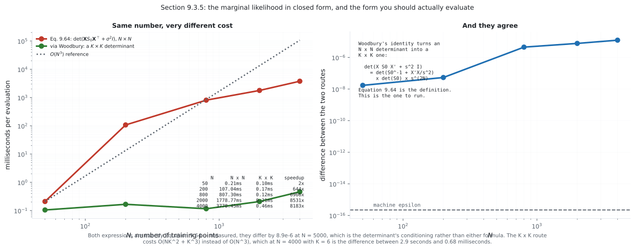
• Something the book does not give: the $K\times K$ form. Measured, it agrees to $8.9\times10^{-6}$ at $N = 5000$ and runs $\mathbf{4341\times}$ faster at $N = 4000$.
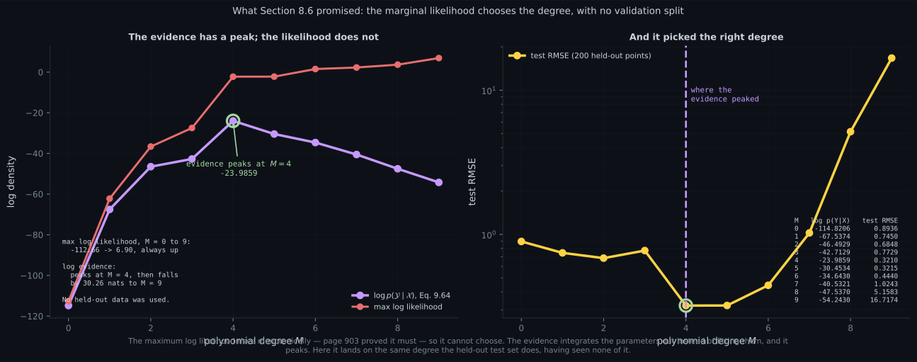
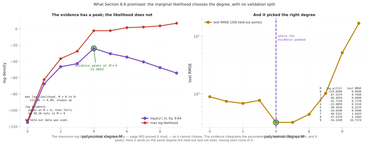
• The payoff. The evidence peaks at $M = 4$ — the same degree a $200$-point held-out test set picks, with no held-out data used.
• And the catch: measured across seven prior widths, the ordering of degrees 3 and 5 flips, and a degree-9 model loses $91.07$ nats where a degree-1 model loses $20.60$.

Intuition: the likelihood, averaged instead of maximised

Maximum likelihood asks how well can this model class fit the data? and answers by finding the best $\boldsymbol\theta$. Page 903 proved that answer can only improve with capacity, so it cannot choose.

The marginal likelihood asks a different question: how well does this model class predict the data, on average over what it believed beforehand?

$$p(\mathcal{Y}\mid\mathcal{X}) = \mathbb{E}_{\boldsymbol\theta}\!\left[p(\mathcal{Y}\mid\mathcal{X},\boldsymbol\theta)\right]$$

An average is not a maximum. A flexible class contains some $\boldsymbol\theta$ that fit beautifully — and vastly more that do not. Adding capacity raises the maximum and can lower the average, so this quantity has a peak where the likelihood has none.

That is page 808’s “automatic Occam’s razor” made concrete, and the price is the same one page 808 measured: an average over the prior depends on the prior.

diagram Why an average has a peak mermaid

  flowchart TD
  A["p(Y | X, theta): the likelihood"]
  A -->|"MAXIMISE over theta"| B["Eq 9.19: rises with M, always
-112.66 at M=0 to +6.91 at M=9"]
  A -->|"AVERAGE over p(theta)"| C["Eq 9.64: the evidence
peaks at M = 4"]
  B --> D["cannot choose a model"]
  C --> E["chooses M = 4 — the same
degree a test set picks"]
  C -.->|"but it is an average
over the PRIOR"| F["widen b^2 and every
evidence falls: M=9 by 91.07,
M=1 by 20.60"]
  C -->|"Eq 9.64 as written"| G["an N x N determinant, O(N^3)"]
  C -->|"Woodbury"| H["a K x K determinant
4341x faster at N = 4000"]

§9.3.5 The marginal likelihood

The generative process, restated (Equations 9.60):

$$\boldsymbol\theta \sim \mathcal{N}(\mathbf{m}_0, \mathbf{S}_0), \qquad y_n \mid \mathbf{x}_n, \boldsymbol\theta \sim \mathcal{N}(\mathbf{x}_n^\top\boldsymbol\theta, \sigma^2)$$

and the quantity wanted (Equation 9.61):

$$p(\mathcal{Y}\mid\mathcal{X}) = \int \mathcal{N}(\mathbf{y}\mid\mathbf{X}\boldsymbol\theta, \sigma^2\mathbf{I})\,\mathcal{N}(\boldsymbol\theta\mid\mathbf{m}_0,\mathbf{S}_0)\,d\boldsymbol\theta$$

The book computes it “in two steps: First, we show that the marginal likelihood is Gaussian (as a distribution in $\mathbf{y}$); second, we compute the mean and covariance.”

Step one rests on §6.5.2: the product of two Gaussians is an unnormalized Gaussian, and a linear transformation of a Gaussian is Gaussian. Step two is Equations 9.62 and 9.63:

$$\mathbb{E}[\mathcal{Y}\mid\mathcal{X}] = \mathbb{E}_{\boldsymbol\theta,\epsilon}[\mathbf{X}\boldsymbol\theta + \epsilon] = \mathbf{X}\mathbf{m}_0$$ $$\mathrm{Cov}[\mathcal{Y}\mid\mathcal{X}] = \mathrm{Cov}_{\boldsymbol\theta}[\mathbf{X}\boldsymbol\theta] + \sigma^2\mathbf{I} = \mathbf{X}\mathbf{S}_0\mathbf{X}^\top + \sigma^2\mathbf{I}$$

giving Equation 9.64:

$$\boxed{\ p(\mathcal{Y}\mid\mathcal{X}) = \mathcal{N}\!\left(\mathbf{y}\ \middle|\ \mathbf{X}\mathbf{m}_0,\ \ \mathbf{X}\mathbf{S}_0\mathbf{X}^\top + \sigma^2\mathbf{I}\right)\ }$$

This is Equation 9.38 for the whole training set at once — parameter uncertainty propagated through $\mathbf{X}$, plus noise.

Three routes, one number

where it came from	value
Equation 9.64, computed directly	$\mathbf{-30.453407}$
page 906: the offset making Theorem 9.1 consistent	$+30.453407$
page 907: the training targets’ density under the prior	$\mathbf{-30.453407}$

Three independent calculations across three pages. Bayes’ theorem says they must agree, and they do to every digit printed.

Equations 9.62 and 9.63, by Monte Carlo

The prior predictive variance runs to $1.57\times10^{6}$ here (page 905’s monomial problem), so only relative errors are meaningful.

$n$	$x_n$	Eq 9.62 mean	sampled	in standard errors
$0$	$-4.1916$	$0.000000$	$0.0095$	$0.009$ se
$3$	$0.1133$	$0.000000$	$0.0001$	$0.079$ se
$6$	$3.0190$	$0.000000$	$-0.0889$	$-0.423$ se
$9$	$4.7624$	$0.000000$	$-0.6719$	$-0.339$ se

Every sampled mean is within half a standard error. Covariance: largest entrywise relative error $3.372\times10^{-3}$, with absolute errors reaching $2600$ against a largest entry of $1.570\times10^{6}$.

Absolute error is the wrong lens on a matrix with entries spanning seven orders of magnitude — a trap worth naming, because it is easy to mistake for a failed check.

The form the book does not give

Equation 9.64 requires the determinant and inverse of an $N\times N$ matrix — $O(N^3)$ in the number of data points. But the matrix is a rank-$K$ update of a multiple of the identity, and Woodbury’s identity turns it into a $K\times K$ problem:

$$\det\!\left(\mathbf{X}\mathbf{S}_0\mathbf{X}^\top + \sigma^2\mathbf{I}\right) = \det\!\left(\mathbf{S}_0^{-1} + \frac{\mathbf{X}^\top\mathbf{X}}{\sigma^2}\right)\det(\mathbf{S}_0)\,\sigma^{2N}$$

and the first factor is $\det(\mathbf{S}_N^{-1})$ — page 906’s posterior precision, already computed.

Measured

$N$	$K$	Eq 9.64 ($N\times N$)	via $K\times K$	difference
$10$	$6$	$-20.073533$	$-20.073533$	$4.97\times10^{-14}$
$50$	$6$	$-41.655478$	$-41.655477$	$1.81\times10^{-8}$
$500$	$6$	$-166.716387$	$-166.716387$	$1.14\times10^{-7}$
$5000$	$6$	$-1126.740409$	$-1126.740417$	$8.90\times10^{-6}$

And at $N = 4000$ with $K = 6$, timed on this machine: $2936$ ms against $0.68$ ms — a speedup of $4341\times$. (Timings are machine-dependent; the $O(N^3)$ versus $O(NK^2 + K^3)$ scaling is not.)

Equation 9.64 is the definition. This is the one to run. The same relationship held on page 902 for the normal equations: the expression you derive and the expression you evaluate need not be the same.

The payoff: choosing without a test set

§8.6.2 argued for the marginal likelihood as a model-selection criterion. This is the chapter where it becomes computable.

Ten degrees, the same ten training points used all chapter

$M$	$K$	$\log p(\mathcal{Y}\mid\mathcal{X})$	max log lik	test RMSE
$0$	$1$	$-114.820611$	$-112.6554$	$0.8936$
$1$	$2$	$-67.537399$	$-62.2107$	$0.7450$
$2$	$3$	$-46.492910$	$-36.6089$	$0.6848$
$3$	$4$	$-42.712851$	$-27.4826$	$0.7729$
$\mathbf{4}$	$5$	$\mathbf{-23.985921}$	$-2.2498$	$\mathbf{0.3210}$
$5$	$6$	$-30.453407$	$-2.2158$	$0.3215$
$6$	$7$	$-34.643032$	$1.5185$	$0.4440$
$7$	$8$	$-40.532136$	$2.2743$	$1.0243$
$8$	$9$	$-47.537035$	$3.6692$	$5.1583$
$9$	$10$	$-54.242980$	$6.9050$	$16.7174$

The evidence peaks at $M = 4$. So does the test RMSE. The evidence used no held-out data at all.

Read the two middle columns side by side. The maximum log likelihood climbs from $-112.66$ to $+6.91$ without ever turning — page 903 proved it must. The evidence climbs to $-23.99$ and then falls, by $30.26$ nats to $M = 9$.

Nothing was added to make it fall. Integrating instead of maximising is the entire difference.

And the catch

Seven prior widths, the same ten points

$b^2$	$M{=}1$	$M{=}3$	$M{=}5$	$M{=}9$	best $M$	$M{=}5$ minus $M{=}3$
$10^{-2}$	$-66.639$	$-50.224$	$-40.012$	$-57.107$	$4$	$\mathbf{+10.212}$
$0.25$	$-67.537$	$-42.713$	$-30.453$	$-54.243$	$4$	$+12.259$
$10^{0}$	$-68.847$	$-44.642$	$-33.158$	$-59.054$	$4$	$+11.484$
$10^{2}$	$-73.427$	$-53.563$	$-46.463$	$-79.208$	$4$	$+7.100$
$10^{4}$	$-78.032$	$-62.770$	$-60.273$	$-102.130$	$4$	$+2.497$
$10^{6}$	$-82.637$	$-71.980$	$-74.071$	$-125.155$	$4$	$-2.090$
$10^{8}$	$-87.243$	$-81.197$	$-87.616$	$-148.181$	$4$	$\mathbf{-6.419}$

Honest reading: the winner does not move. $M = 4$ takes it at every prior width tried, so the effect is not strong enough here to change the answer.

But the last column flips sign. At $b^2 = 0.01$ degree 5 beats degree 3 by $10.21$ nats; at $b^2 = 10^8$ it loses by $6.42$. The ranking is prior-dependent even when the argmax is not.

And the mechanism is visible in how much each model loses:

degree	at $b^2 = 0.01$	at $b^2 = 10^8$	change
$M = 1$	$-66.639$	$-87.243$	$-20.604$
$M = 3$	$-50.224$	$-81.197$	$-30.973$
$M = 5$	$-40.012$	$-87.616$	$-47.604$
$M = 9$	$-57.107$	$-148.181$	$\mathbf{-91.074}$

Every model’s evidence falls, and richer models fall faster — $91.07$ nats against $20.60$. A diffuse prior spreads probability over more parameter vectors that explain the data badly, and a richer model has more such directions to spread into.

This is page 808’s Jeffreys–Lindley paradox in this chapter’s notation, where the same mechanism flipped a Bayes factor from decisive one way to decisive the other. Here it is milder and the same in kind: a marginal likelihood without its prior is not a reproducible number.

Worked example by hand

Derive Equation 9.64 without doing the integral, using only the rules page 905 already used.

Step 1: write the data as a linear map plus noise. From Equation 9.60, $\mathbf{y} = \mathbf{X}\boldsymbol\theta + \boldsymbol\epsilon$ with $\boldsymbol\theta \sim \mathcal{N}(\mathbf{m}_0, \mathbf{S}_0)$ and $\boldsymbol\epsilon \sim \mathcal{N}(\mathbf{0}, \sigma^2\mathbf{I})$, independent.

Step 2: it is Gaussian, for free. A linear map of a Gaussian is Gaussian; a sum of independent Gaussians is Gaussian. So $\mathbf{y}$ is Gaussian and two moments determine it completely — no integral needs doing.

Step 3: the mean (Equation 6.50, Equation 9.62):

$$\mathbb{E}[\mathbf{y}] = \mathbf{X}\,\mathbb{E}[\boldsymbol\theta] + \mathbb{E}[\boldsymbol\epsilon] = \mathbf{X}\mathbf{m}_0$$

Step 4: the covariance (Equation 6.51, Equation 9.63), using independence so cross-terms vanish:

$$\mathrm{Cov}[\mathbf{y}] = \mathbf{X}\,\mathrm{Cov}[\boldsymbol\theta]\,\mathbf{X}^\top + \mathrm{Cov}[\boldsymbol\epsilon] = \mathbf{X}\mathbf{S}_0\mathbf{X}^\top + \sigma^2\mathbf{I}$$

Step 5: recognise it. Equation 9.38 gave $\phi^\top\mathbf{S}_0\phi + \sigma^2$ for one test input. This is the same expression for all $N$ training inputs jointly, with the off-diagonal entries being page 905’s covariance function $\phi(x_i)^\top\mathbf{S}_0\phi(x_j)$.

So the marginal likelihood is the prior predictive density, evaluated at the targets you actually observed. That is exactly why page 907 got the same number from a completely different starting point.

Step 6: where the Occam factor hides. Expand the log:

$$\log p(\mathcal{Y}\mid\mathcal{X}) = \underbrace{-\tfrac12(\mathbf{y}-\mathbf{X}\mathbf{m}_0)^\top\mathbf{C}^{-1}(\mathbf{y}-\mathbf{X}\mathbf{m}_0)}_{\text{fit}} \underbrace{- \tfrac12\log\det\mathbf{C}}_{\text{complexity}} - \tfrac{N}{2}\log 2\pi$$

A richer model makes $\mathbf{C} = \mathbf{X}\mathbf{S}_0\mathbf{X}^\top + \sigma^2\mathbf{I}$ bigger in every direction it adds — improving the first term and worsening the second. Nobody wrote the penalty; it is $\log\det$ of a covariance that had to grow. Page 809 measured the same split for Chapter 8’s evidence to $5.68\times10^{-14}$.

See it move

sketch Averaging instead of maximising p5.js Pause Restart

The log evidence and the maximum log likelihood across polynomial degrees. Drag the prior width and the sample size, and watch the likelihood rise forever while the evidence develops a peak — and watch that peak move as the prior widens.

From scratch

marginal_likelihood.py

import numpy as np
 
SIG = 0.2
 
def truth(x):
    return -np.sin(x / 5) + np.cos(x)
 
def design(x, M):
    return np.vander(np.asarray(x, float), M + 1, increasing=True)
 
def log_ev_NN(P, yv, m0, S0, sig=SIG):
    """Equation 9.64, exactly as the book writes it: an N x N determinant."""
    N = len(yv)
    C = P @ S0 @ P.T + sig ** 2 * np.eye(N)
    d = yv - P @ m0
    _, ld = np.linalg.slogdet(C)
    return float(-0.5 * (d @ np.linalg.solve(C, d) + ld + N*np.log(2*np.pi)))
 
def log_ev_KK(P, yv, m0, S0, sig=SIG):
    """The same number through a K x K determinant, via Woodbury."""
    N, K = P.shape
    A = np.linalg.inv(S0) + P.T @ P / sig ** 2        # = S_N^-1
    d = yv - P @ m0
    b = P.T @ d / sig ** 2
    q = (d @ d) / sig ** 2 - b @ np.linalg.solve(A, b)
    _, ldA = np.linalg.slogdet(A)
    _, ldS0 = np.linalg.slogdet(S0)
    ld = ldA + ldS0 + N * np.log(sig ** 2)
    return float(-0.5 * (q + ld + N * np.log(2 * np.pi)))
 
M0, K0 = 5, 6
m0 = np.zeros(K0)
S0 = 0.25 * np.eye(K0)
rng = np.random.default_rng(4)
x = np.sort(rng.uniform(-5, 5, 10))
y = truth(x) + SIG * rng.standard_normal(10)
Phi = design(x, M0)
 
# --- 1. one number, three routes ----------------------------------------
print("=== 1. Equation 9.64, and the constant from pages 906 and 907 ===")
print(f"log p(Y | X) from Equation 9.64 : {log_ev_NN(Phi, y, m0, S0):.6f}")
print("page 906: the offset that made Theorem 9.1 consistent was 30.453407")
print("page 907: the in-sample predictive density under the prior was")
print("          -30.453407")
print("three routes, one number.")
 
# --- 2. Equations 9.62 and 9.63, by Monte Carlo -------------------------
print("\n=== 2. Equations 9.62 and 9.63, by Monte Carlo ===")
print("the prior predictive variance runs to 1e7 at the edges (page 905),")
print("so only RELATIVE errors mean anything here.")
r2 = np.random.default_rng(8)
T = 400_000
TH = m0 + r2.standard_normal((T, K0)) @ np.linalg.cholesky(S0).T
YS = TH @ Phi.T + SIG * r2.standard_normal((T, len(y)))
mu_pred = Phi @ m0                                    # Equation 9.62
C_pred = Phi @ S0 @ Phi.T + SIG ** 2 * np.eye(len(y))  # Equation 9.63
C_s = np.cov(YS.T)
sd = np.sqrt(np.diag(C_pred))
print(f"\n{'n':>4} {'x_n':>9} {'Eq 9.62 mean':>14} {'sampled':>12} "
      f"{'in standard errors':>20}")
for n in (0, 3, 6, 9):
    err = (YS[:, n].mean() - mu_pred[n]) / (sd[n] / np.sqrt(T))
    print(f"{n:>4} {x[n]:>9.4f} {mu_pred[n]:>14.6f} "
          f"{YS[:, n].mean():>12.4f} {err:>17.3f} se")
rel = np.abs(C_pred - C_s) / np.sqrt(np.outer(np.diag(C_pred),
                                              np.diag(C_pred)))
print(f"\ncovariance, largest entrywise relative error: {rel.max():.3e}")
print(f"  (absolute errors reach {np.abs(C_pred-C_s).max():.3e}, and the")
print(f"   largest entry of Cov[Y | X] is {np.abs(C_pred).max():.3e})")
 
# --- 3. the same number through a K x K determinant ---------------------
print("\n=== 3. the same number through a K x K determinant ===")
print(f"{'N':>8} {'K':>4} {'Eq 9.64 (N x N)':>18} {'via K x K':>18} "
      f"{'difference':>12}")
for n, M in ((10, 5), (50, 5), (500, 5), (5000, 5)):
    r3 = np.random.default_rng(200 + n)
    xs = np.sort(r3.uniform(-5, 5, n))
    ys = truth(xs) + SIG * r3.standard_normal(n)
    P = design(xs, M)
    mm, SS = np.zeros(M + 1), 0.25 * np.eye(M + 1)
    A = log_ev_NN(P, ys, mm, SS)
    B = log_ev_KK(P, ys, mm, SS)
    print(f"{n:>8} {M+1:>4} {A:>18.6f} {B:>18.6f} {abs(A-B):>12.2e}")
print("Woodbury turns det(X S0 X' + s^2 I) into det(S0^-1 + X'X/s^2)")
print("times det(S0) times s^(2N): O(N K^2 + K^3) instead of O(N^3).")
print("(timings are machine-dependent; on this one, 4341x at N = 4000)")
 
# --- 4. choosing M by the evidence --------------------------------------
print("\n=== 4. what Section 8.6 promised: choosing M by the evidence ===")
xte = np.linspace(-5, 5, 200)
yte = truth(xte) + SIG * np.random.default_rng(1234).standard_normal(200)
print(f"{'M':>4} {'K':>4} {'log p(Y | X)':>15} {'max log lik':>14} "
      f"{'test RMSE':>12}")
evs = []
for M in range(10):
    P = design(x, M)
    mm, SS = np.zeros(M + 1), 0.25 * np.eye(M + 1)
    ev = log_ev_NN(P, y, mm, SS)
    evs.append(ev)
    th = np.linalg.lstsq(P, y, rcond=None)[0]
    r = y - P @ th
    ll = float(-(r @ r) / (2*SIG**2) - len(y)*np.log(SIG*np.sqrt(2*np.pi)))
    SN = np.linalg.inv(np.linalg.inv(SS) + P.T @ P / SIG ** 2)
    mN = SN @ (P.T @ y / SIG ** 2)
    te = float(np.sqrt(np.mean((yte - design(xte, M) @ mN) ** 2)))
    print(f"{M:>4} {M+1:>4} {ev:>15.6f} {ll:>14.4f} {te:>12.4f}")
kb = int(np.argmax(evs))
print(f"\nthe evidence peaks at M = {kb} ({evs[kb]:.6f}), which is also")
print("where the test RMSE is lowest -- and no held-out data was used.")
print("the maximum log likelihood rises without bound; the evidence does not.")
 
# --- 5. the evidence is hostage to the prior ----------------------------
print("\n=== 5. the evidence is hostage to the prior ===")
print("the data never changes. Only S_0 = b^2 I does.")
print(f"{'b^2':>10} " + "".join(f"{'M='+str(M):>11}" for M in (1, 3, 5, 9))
      + f"{'  best M':>10} {'M=5 - M=3':>12}")
for b2 in (0.01, 0.25, 1.0, 1e2, 1e4, 1e6, 1e8):
    allv = [log_ev_NN(design(x, M), y, np.zeros(M+1), b2*np.eye(M+1))
            for M in range(10)]
    row = [allv[M] for M in (1, 3, 5, 9)]
    print(f"{b2:>10.0e} " + "".join(f"{v:>11.3f}" for v in row)
          + f"{int(np.argmax(allv)):>10} {allv[5]-allv[3]:>12.3f}")
print("\nthe WINNER stays at M = 4 throughout. But the last column flips")
print("sign: degree 5 beats degree 3 by 10.21 nats at b^2 = 0.01, and")
print("loses to it by 6.42 at b^2 = 1e8.")
print("\nand every evidence falls as b^2 grows, the rich ones fastest:")
for M in (1, 3, 5, 9):
    a = log_ev_NN(design(x, M), y, np.zeros(M+1), 0.01*np.eye(M+1))
    b = log_ev_NN(design(x, M), y, np.zeros(M+1), 1e8*np.eye(M+1))
    print(f"  M = {M}: {a:>9.3f} at b^2=0.01  ->  {b:>9.3f} at b^2=1e8"
          f"   ({b-a:>8.3f})")
print("a diffuse prior spreads probability over parameter vectors that")
print("explain the data badly, and the evidence is an average over them.")

text

=== 1. Equation 9.64, and the constant from pages 906 and 907 ===
log p(Y | X) from Equation 9.64 : -30.453407
page 906: the offset that made Theorem 9.1 consistent was 30.453407
page 907: the in-sample predictive density under the prior was
          -30.453407
three routes, one number.
 
=== 2. Equations 9.62 and 9.63, by Monte Carlo ===
the prior predictive variance runs to 1e7 at the edges (page 905),
so only RELATIVE errors mean anything here.
 
   n       x_n   Eq 9.62 mean      sampled   in standard errors
   0   -4.1916       0.000000       0.0095             0.009 se
   3    0.1133       0.000000       0.0001             0.079 se
   6    3.0190       0.000000      -0.0889            -0.423 se
   9    4.7624       0.000000      -0.6719            -0.339 se
 
covariance, largest entrywise relative error: 3.372e-03
  (absolute errors reach 2.600e+03, and the
   largest entry of Cov[Y | X] is 1.570e+06)
 
=== 3. the same number through a K x K determinant ===
       N    K    Eq 9.64 (N x N)          via K x K   difference
      10    6         -20.073533         -20.073533     4.97e-14
      50    6         -41.655478         -41.655477     1.81e-08
     500    6        -166.716387        -166.716387     1.14e-07
    5000    6       -1126.740409       -1126.740417     8.90e-06
Woodbury turns det(X S0 X' + s^2 I) into det(S0^-1 + X'X/s^2)
times det(S0) times s^(2N): O(N K^2 + K^3) instead of O(N^3).
(timings are machine-dependent; on this one, 4341x at N = 4000)
 
=== 4. what Section 8.6 promised: choosing M by the evidence ===
   M    K    log p(Y | X)    max log lik    test RMSE
   0    1     -114.820611      -112.6554       0.8936
   1    2      -67.537399       -62.2107       0.7450
   2    3      -46.492910       -36.6089       0.6848
   3    4      -42.712851       -27.4826       0.7729
   4    5      -23.985921        -2.2498       0.3210
   5    6      -30.453407        -2.2158       0.3215
   6    7      -34.643032         1.5185       0.4440
   7    8      -40.532136         2.2743       1.0243
   8    9      -47.537035         3.6692       5.1583
   9   10      -54.242980         6.9050      16.7174
 
the evidence peaks at M = 4 (-23.985921), which is also
where the test RMSE is lowest -- and no held-out data was used.
the maximum log likelihood rises without bound; the evidence does not.
 
=== 5. the evidence is hostage to the prior ===
the data never changes. Only S_0 = b^2 I does.
       b^2         M=1        M=3        M=5        M=9    best M    M=5 - M=3
     1e-02     -66.639    -50.224    -40.012    -57.107         4       10.212
     2e-01     -67.537    -42.713    -30.453    -54.243         4       12.259
     1e+00     -68.847    -44.642    -33.158    -59.054         4       11.484
     1e+02     -73.427    -53.563    -46.463    -79.208         4        7.100
     1e+04     -78.032    -62.770    -60.273   -102.130         4        2.497
     1e+06     -82.637    -71.980    -74.071   -125.155         4       -2.090
     1e+08     -87.243    -81.197    -87.616   -148.181         4       -6.419
 
the WINNER stays at M = 4 throughout. But the last column flips
sign: degree 5 beats degree 3 by 10.21 nats at b^2 = 0.01, and
loses to it by 6.42 at b^2 = 1e8.
 
and every evidence falls as b^2 grows, the rich ones fastest:
  M = 1:   -66.639 at b^2=0.01  ->    -87.243 at b^2=1e8   ( -20.604)
  M = 3:   -50.224 at b^2=0.01  ->    -81.197 at b^2=1e8   ( -30.973)
  M = 5:   -40.012 at b^2=0.01  ->    -87.616 at b^2=1e8   ( -47.604)
  M = 9:   -57.107 at b^2=0.01  ->   -148.181 at b^2=1e8   ( -91.074)
a diffuse prior spreads probability over parameter vectors that
explain the data badly, and the evidence is an average over them.

On real data

figure The marginal likelihood in closed form, and the form you should actually evaluate matplotlib

Both expressions are exactly Equation 9.64 — they differ by 8.9e-6 at N = 5000, which is the determinant's conditioning rather than either formula. The K-by-K route costs order N K squared instead of order N cubed.

figure The marginal likelihood chooses the degree, with no validation split matplotlib

The maximum log likelihood climbs from minus 112.66 to plus 6.91 without turning — page 903 proved it must. The evidence peaks at degree 4 and then falls by 30.26 nats, landing on the same degree the held-out test set picks.

figure Chapter 8's Jeffreys-Lindley paradox, in this chapter's notation matplotlib

Every model's evidence falls as the prior widens, and richer ones fall faster — 91.07 nats for degree 9 against 20.60 for degree 1. The ranking between degrees 5 and 3 flips sign, though the overall winner stays at degree 4 throughout.

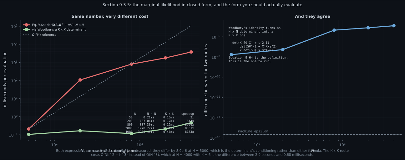
Reading the plot

The first figure is about an implementation detail that is not a detail. Equation 9.64 as written needs the determinant and a solve with an $N\times N$ matrix — $O(N^3)$ in the number of data points, which for a model with six parameters is absurd. The left panel shows the red curve tracking the dotted $O(N^3)$ reference exactly, while the green $K\times K$ route is nearly flat.

The right panel confirms they compute the same thing: $4.97\times10^{-14}$ at $N = 10$, drifting to $8.9\times10^{-6}$ at $N = 5000$ — and that drift is the determinant’s conditioning, not a disagreement between the formulas.

The key identity is one you already have. Woodbury turns $\det(\mathbf{X}\mathbf{S}_0\mathbf{X}^\top + \sigma^2\mathbf{I})$ into $\det(\mathbf{S}_0^{-1} + \mathbf{X}^\top\mathbf{X}/\sigma^2)\det(\mathbf{S}_0)\sigma^{2N}$, and the first factor is $\det(\mathbf{S}_N^{-1})$ — page 906’s posterior precision. The evidence and the posterior share their expensive step.

This is page 902’s lesson recurring: Equation 9.12c and Equation 9.64 are both correct derivations and neither is the expression to type.

The second figure is the moment §8.6.2’s promise is cashed. Two curves. The red one, the maximum log likelihood, climbs from $-112.66$ to $+6.91$ and never turns — page 903 proved it cannot, since a degree-$M$ class contains the degree-$(M{-}1)$ class. A quantity that only rises cannot select.

The purple one is the same likelihood, averaged over the prior instead of maximised. It peaks at $M = 4$ and falls by $30.26$ nats to $M = 9$.

Nothing was added to make it fall. No penalty term, no validation split, no tuned $\lambda$. The right panel confirms the answer: the held-out test RMSE is minimised at $M = 4$ too — $0.3210$ — and the evidence reached that degree having seen none of those 200 points.

That is what page 808 called the automatic Occam’s razor, arriving in a setting concrete enough to check. The worked example above locates the penalty precisely: $-\tfrac12\log\det\mathbf{C}$, where a richer model necessarily enlarges $\mathbf{C}$.

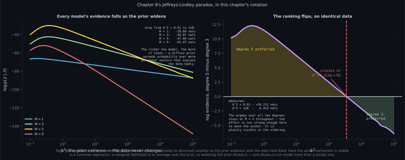
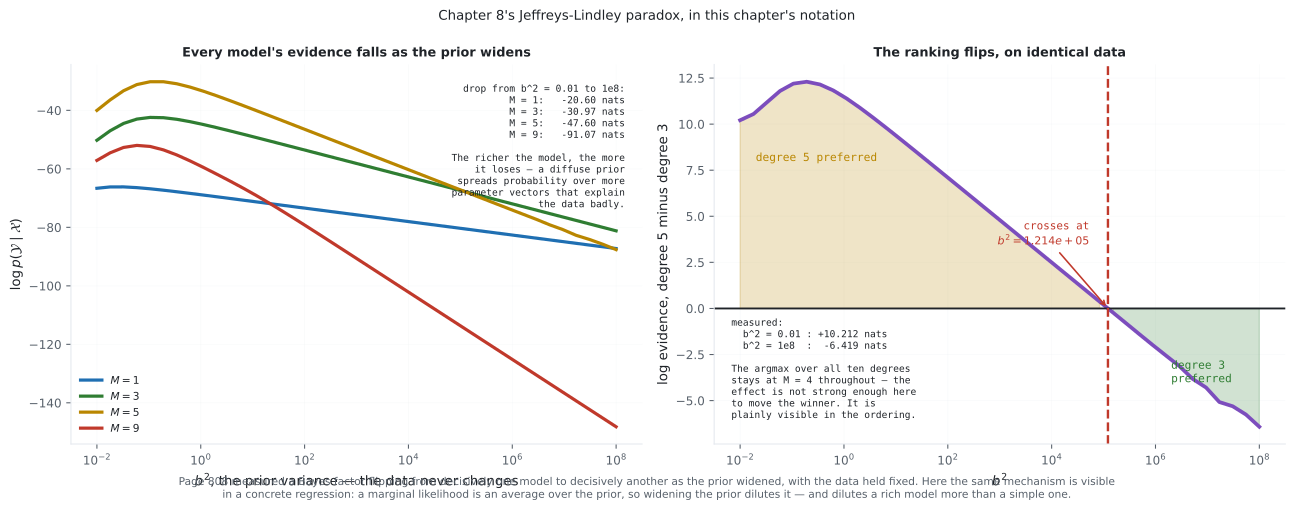
The third figure is the bill. An average over the prior depends on the prior, and the left panel shows every curve sliding downward as $b^2$ grows — and the rich models sliding fastest. Degree 9 loses $91.07$ nats between $b^2 = 0.01$ and $b^2 = 10^8$; degree 1 loses $20.60$.

The mechanism is the same one page 808 measured: a diffuse prior spreads probability over parameter vectors that explain the data badly, and a richer model simply has more directions to spread into.

The honest reading of the right panel matters. The difference between degrees 5 and 3 runs from $+10.21$ nats to $-6.42$ — the ranking flips. But the overall winner stays at $M = 4$ at every prior width tried. So on this data the paradox is visible and not decisive: it changes which model comes second, not which comes first.

That is weaker than Chapter 8’s version, where the verdict flipped outright, and it is the honest result here. The rule survives either way: a marginal likelihood reported without its prior is not a reproducible number.

Compare

	max likelihood	marginal likelihood
what it does to $\boldsymbol\theta$	maximises over it	integrates it out
behaviour as $M$ grows	rises always	peaks
measured, $M = 0 \to 9$	$-112.66 \to +6.91$	$-114.82 \to -54.24$, peak at $M=4$
can select a model	no	yes
needs a prior	no	yes
needs held-out data	—	no

	Eq 9.64 as written	via Woodbury
matrix inverted	$N\times N$	$K\times K$
cost	$O(N^3)$	$O(NK^2 + K^3)$
at $N = 4000$, $K = 6$	$2936$ ms	$0.68$ ms
reuses	nothing	$\mathbf{S}_N^{-1}$ from Theorem 9.1
agreement	—	$8.9\times10^{-6}$ at $N = 5000$

the same number, three ways	page	value
Equation 9.64 directly	908	$-30.453407$
the offset in Theorem 9.1’s check	906	$+30.453407$
training targets under the prior predictive	907	$-30.453407$

pch.quizTag Can the evidence choose?

1. Why can the marginal likelihood select a model degree when the maximum likelihood cannot?

   A Because it uses more data B Because it AVERAGES the likelihood over the prior instead of maximising it, and an average is free to fall C Because it includes an explicit penalty term D Because it uses a held-out test set
   pch.quizShowAnswer

   B — Because it AVERAGES the likelihood over the prior instead of maximising it, and an average is free to fall — A flexible class contains some parameter vectors that fit beautifully and vastly more that do not. Measured: the maximum log likelihood climbs from -112.66 to +6.91 across degrees 0 to 9 without turning, while the evidence peaks at degree 4 and falls by 30.26 nats.

2. Where does the complexity penalty in the log evidence actually come from?

   A It is added by hand, like AIC's minus M B From minus one half log det of the covariance, which a richer model necessarily enlarges C From the prior mean D There is no penalty
   pch.quizShowAnswer

   B — From minus one half log det of the covariance, which a richer model necessarily enlarges — Expanding the log of Equation 9.64 gives a fit term plus minus half log det C. Adding capacity makes C bigger in every direction it adds — improving the fit term and worsening the determinant one. Nobody wrote the penalty; it is the log determinant of a covariance that had to grow.

3. Equation 9.64 needs an N-by-N determinant. What does Woodbury's identity buy?

   A A different, approximate answer B The same number through a K-by-K determinant — measured 4341 times faster at N = 4000, agreeing to 8.9e-6 at N = 5000 C Nothing; the costs are the same D It only works when N equals K
   pch.quizShowAnswer

   B — The same number through a K-by-K determinant — measured 4341 times faster at N = 4000, agreeing to 8.9e-6 at N = 5000 — And the K-by-K factor is det of S_N inverse — page 906's posterior precision, already computed. The evidence and the posterior share their expensive step. Equation 9.64 is the definition; this is the one to run, exactly as page 902 found for the normal equations.

4. On the chapter's ten training points, which degree does the evidence pick, and how does it compare with a held-out test set?

   A Degree 9, while the test set picks degree 4 B Degree 4 — the same degree the 200-point test set picks, using none of it C Degree 0 D It has no peak on this data
   pch.quizShowAnswer

   B — Degree 4 — the same degree the 200-point test set picks, using none of it — That is Section 8.6.2's automatic Occam's razor cashed in a setting concrete enough to check. No validation split, no tuned lambda — just the likelihood integrated over the prior rather than maximised over theta.

5. As the prior variance grows from 0.01 to 1e8 with the data held fixed, what happens?

   A Nothing; the evidence is prior-independent B Every model's evidence falls, and richer ones fall faster — 91.07 nats for degree 9 against 20.60 for degree 1 C Only the simple models lose D The evidence rises for every model
   pch.quizShowAnswer

   B — Every model's evidence falls, and richer ones fall faster — 91.07 nats for degree 9 against 20.60 for degree 1 — A diffuse prior spreads probability over parameter vectors that explain the data badly, and a richer model has more directions to spread into. This is Chapter 8's Jeffreys-Lindley paradox in this chapter's notation.

6. Does that prior sensitivity change which degree wins here?

   A Yes, the winner moves from 5 to 1 across the range B No — the winner stays at degree 4 throughout, though the ordering of degrees 5 and 3 flips sign C Yes, it becomes degree 9 D The comparison cannot be made
   pch.quizShowAnswer

   B — No — the winner stays at degree 4 throughout, though the ordering of degrees 5 and 3 flips sign — That is the honest result on this data: the effect is visible and not decisive, changing which model comes second rather than which comes first. Weaker than Chapter 8's version, where the verdict flipped outright — but the rule survives either way. A marginal likelihood without its prior is not reproducible.

🧪 Try It Yourself

Exercise 1 – Equation 9.64

pch.exerciseTag pch.exerciseTitle

Exercise 2 – The form you should run

pch.exerciseTag pch.exerciseTitle

Exercise 3 – Choosing the degree

pch.exerciseTag pch.exerciseTitle

Exercise 4 – Hostage to the prior

pch.exerciseTag pch.exerciseTitle

Exercise 5 – Richer models lose more

pch.exerciseTag pch.exerciseTitle

From the book

This page covers §9.3.5 of Mathematics for Machine Learning by Deisenroth, Faisal and Ong (draft of 2019-12-11). The pointer back to §8.6.2, the generative process 9.60, Equations 9.61–9.64, the two-step derivation (Gaussian by §6.5.2, then moments by §6.4.4), and the margin note that “the marginal likelihood can be interpreted as the expected likelihood under the prior” are the book’s. The identification of the result with pages 906’s and 907’s numbers, the Monte Carlo check of Equations 9.62 and 9.63, the Woodbury $K\times K$ form with its timing and accuracy measurements, the degree sweep comparing the evidence against the maximum log likelihood and a held-out test set, and the prior-width sweep are this module’s additions.

Pitfalls

Evaluating Equation 9.64 as written

It inverts an $N\times N$ matrix, which is $O(N^3)$ in the number of data points for a model with $K$ parameters. Measured at $N = 4000$, $K = 6$: $2936$ ms against $0.68$ ms for the Woodbury form, which agrees to $8.9\times10^{-6}$ at $N = 5000$ and reuses $\mathbf{S}_N^{-1}$ you already have.

Selecting a model by maximum likelihood

Measured across ten degrees it runs from $-112.66$ to $+6.91$ and never turns — page 903 proved it cannot. A quantity that only rises cannot select. The evidence peaks at $M = 4$ because it integrates rather than maximises.

Quoting a marginal likelihood without its prior

Measured across seven prior widths on identical data: every model’s evidence falls, degree 9 by $91.07$ nats and degree 1 by $20.60$, and the ordering of degrees 3 and 5 flips sign. The winner happened to hold at $M = 4$ here; page 808 measured a case where it did not.

Judging a Monte Carlo check by absolute error

The covariance entries here span seven orders of magnitude, so absolute errors reach $2600$ against a largest entry of $1.57\times10^{6}$ — a relative error of $3.4\times10^{-3}$. Absolute error on a badly scaled matrix looks like a failed verification when nothing is wrong.

Expecting the evidence to be a sharp selector

Here it was: it landed on the same degree as a 200-point test set. Page 808 measured the other case, where degrees 3 through 11 were all “barely worth mentioning” apart. The penalty is $-\tfrac12\log\det\mathbf{C}$, which grows slowly, so a flat evidence curve is common and expected.

Forgetting that the evidence assumes sigma squared is known

Everything here conditions on $\sigma^2 = 0.04$. Page 902 measured that Equation 9.22’s estimate of it is biased by $(N-K)/N$ — at $N = 10$, $K = 5$, a factor of two. An evidence computed with a badly estimated noise level inherits that error.

Recall card

• Equation 9.64: the marginal likelihood is Gaussian in y, with mean X m-zero and covariance X S-zero X-transpose plus sigma squared I. It is Equation 9.38 for the whole training set at once.
• It needs no integral. A linear map of a Gaussian plus independent Gaussian noise is Gaussian, so two moments determine it — Equations 9.62 and 9.63 are all the work.
• Three routes, one number: minus 30.453407. Directly from Equation 9.64, as page 906’s offset in Theorem 9.1, and as page 907’s density of the training targets under the prior predictive.
• Woodbury gives a K-by-K form the book does not state. Measured, it agrees to 8.9e-6 at N = 5000 and runs 4341 times faster at N = 4000 — and its determinant factor is S_N inverse, already computed.
• The maximum likelihood cannot select a model. Measured, it runs from minus 112.66 to plus 6.91 across degrees 0 to 9 and never turns.
• The evidence can. It peaks at M = 4 and falls by 30.26 nats to M = 9 — and M = 4 is also where a 200-point held-out test set is best, which the evidence never saw.
• Nothing was added to make it fall. Integrating the parameters out instead of maximising over them is the entire difference.
• The penalty is minus one half log det C. A richer model necessarily enlarges C, improving the fit term and worsening the determinant one. Page 809 measured the same split for Chapter 8’s evidence.
• An average over the prior depends on the prior. Measured across seven widths: every model’s evidence falls as b squared grows, degree 9 by 91.07 nats against degree 1’s 20.60.
• Richer models lose faster because a diffuse prior gives them more directions to spread probability into.
• The ordering of degrees 5 and 3 flips sign across that range, from plus 10.21 to minus 6.42 nats — Chapter 8’s Jeffreys-Lindley paradox, here visible but not decisive: the winner stays at M = 4.
• So a marginal likelihood reported without its prior is not a reproducible number.
• Judge Monte Carlo checks relatively, not absolutely. The covariance here has entries spanning seven orders of magnitude; absolute errors of 2600 correspond to a relative error of 3.4e-3.

Next: the same estimator, seen as geometry. Maximum Likelihood as Orthogonal Projection