Empirical Risk Minimization

The book’s framing for this section is blunt: “the ‘learning’ part of machine learning boils down to estimating parameters based on training data.” This page is one way to do that, and its distinguishing feature is that no probability distribution ever gets written down.

Empirical risk minimization was popularised by the support vector machine (Chapter 12), but the book is careful that its principles are general — they “allow us to ask the question of what is learning without explicitly constructing probabilistic models.”

What you’ll learn

• The four design choices of §8.2, and which section answers each.
• §8.2.1: the hypothesis class, and why enlarging it can never raise the training risk. Measured: 0 increases in 15 steps.
• §8.2.2: the loss function, the empirical risk of Equation 8.6, and the i.i.d. assumption that licenses using an empirical mean at all.
• Equation 8.9, the least-squares problem in matrix form, and why it has a closed-form answer.
• Equation 8.10, the expected risk — the thing you actually want and can never compute.
• Measured: the training risk falls monotonically to $0.046494$ while the expected risk climbs to $40.077320$, a ratio of 862.
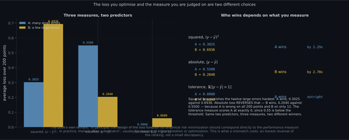
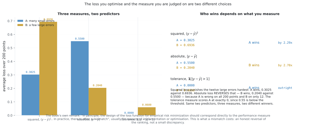
• The book’s closing remark that the loss you optimise is not the measure you are judged on — with two predictors whose ranking reverses between squared and absolute loss.

Intuition: grading yourself on the practice exam

You want a student who does well on the final. You only have the practice questions.

So you grade on the practice questions and hope. That is empirical risk minimization: minimise the average error on the data you have, because the average error on data you do not have is unavailable by definition.

The failure mode is immediate and it is the subject of §8.2.3 and §8.2.4. A student allowed to memorise the practice answers scores perfectly and learns nothing. And you cannot detect this by looking at the practice score — a memoriser and a genius have identical practice scores. The whole problem is that the quantity you can measure and the quantity you care about are different quantities.

diagram Section 8.2's four design choices mermaid

  flowchart TD
  D["training data
(x_1, y_1) ... (x_N, y_N)"]
  Q1["1. what functions may the predictor be?
Section 8.2.1"]
  Q2["2. how do we score it on the training data?
Section 8.2.2"]
  Q3["3. how do we make it generalise?
Section 8.2.3"]
  Q4["4. how do we search the space of models?
Section 8.2.4"]
  D --> Q1 --> Q2 --> RE["R_emp, Eq 8.6
computable"]
  RE --> Q3 --> Q4
  RT["R_true, Eq 8.10
the expectation over ALL data"]
  RE -.->|"underestimates"| RT
  Q3 --> RT
  Q4 --> RT
  style RT stroke-dasharray: 4 3

The dashed node is the point of the whole section. $R_{\text{true}}$ is what “good” means, it is defined as an expectation over an infinite population, and it is not available. Everything else is machinery for coping with that.

§8.2.1 The hypothesis class

Given $N$ examples $\mathbf{x}_n \in \mathbb{R}^D$ with scalar labels $y_n \in \mathbb{R}$, we want a predictor $f(\cdot, \boldsymbol\theta) : \mathbb{R}^D \to \mathbb{R}$ and a good parameter $\boldsymbol\theta^*$ such that

$$f(\mathbf{x}_n, \boldsymbol\theta^*) \approx y_n \quad \text{for all } n = 1, \dots, N$$

Write $\hat{y}_n = f(\mathbf{x}_n, \boldsymbol\theta^*)$ for the predictor’s output.

Example 8.1 picks the class: affine functions. Using the unit-feature trick from §8.1,

$$f(\mathbf{x}_n, \boldsymbol\theta) = \boldsymbol\theta^\top\mathbf{x}_n \qquad\text{which is}\qquad f(\mathbf{x}_n, \boldsymbol\theta) = \theta_0 + \sum_{d=1}^{D}\theta_d x_n^{(d)}$$

so $f : \mathbb{R}^{D+1} \to \mathbb{R}$. Every straight-line predictor in the chapter’s figures is this.

A bigger class can never fit the training data worse

This is worth stating precisely because it is what makes training risk useless for choosing a class. A degree-$d$ polynomial is a degree-$(d+1)$ polynomial with its top coefficient set to zero. So the degree-$(d+1)$ class contains the degree-$d$ class, and its best member is at least as good.

Measured over degrees $0$ to $15$: the training risk decreased at every one of the 15 steps, from $0.993663$ to $0.046494$. Not once did it rise. That monotonicity is not a property of this dataset — it is a property of nested classes, and it holds for any data.

§8.2.2 The loss function, and the empirical risk

A loss function $\ell(y_n, \hat{y}_n)$ takes a label and a prediction and returns a non-negative number. The book notes “error” is often used to mean loss.

Then comes the assumption that makes the whole framework work:

One assumption that is commonly made in machine learning is that the set of examples $(\mathbf{x}_1, y_1), \dots, (\mathbf{x}_N, y_N)$ is independent and identically distributed.

Independence (§6.4.5) means two data points do not statistically depend on each other, which means “the empirical mean is a good estimate of the population mean” (§6.4.1). That is what licenses averaging the loss over the training set rather than doing something more careful.

Stacking examples into $\mathbf{X} := [\mathbf{x}_1, \dots, \mathbf{x}_N]^\top \in \mathbb{R}^{N\times D}$ and labels into $\mathbf{y} := [y_1, \dots, y_N]^\top \in \mathbb{R}^N$:

$$R_{\text{emp}}(f, \mathbf{X}, \mathbf{y}) = \frac{1}{N}\sum_{n=1}^{N}\ell(y_n, \hat{y}_n)$$

This is the empirical risk, and minimising it is empirical risk minimization. Note it depends on three things — the predictor and the data — which is what makes the notation $R_{\text{emp}}(f, \mathbf{X}, \mathbf{y})$ worth carrying: the same $f$ has a different empirical risk on a different dataset, and §8.2.4 exploits exactly that.

Example 8.2: least squares

Take the squared loss $\ell(y_n, \hat{y}_n) = (y_n - \hat{y}_n)^2$. Then

$$\min_{\boldsymbol\theta\in\mathbb{R}^D} \frac{1}{N}\sum_{n=1}^{N}\big(y_n - f(\mathbf{x}_n, \boldsymbol\theta)\big)^2$$

and with the linear predictor $f(\mathbf{x}_n, \boldsymbol\theta) = \boldsymbol\theta^\top\mathbf{x}_n$,

$$\min_{\boldsymbol\theta\in\mathbb{R}^D} \frac{1}{N}\sum_{n=1}^{N}\big(y_n - \boldsymbol\theta^\top\mathbf{x}_n\big)^2 \qquad\text{equivalently}\qquad \min_{\boldsymbol\theta\in\mathbb{R}^D} \frac{1}{N}\lVert\mathbf{y} - \mathbf{X}\boldsymbol\theta\rVert^2$$

This is the least-squares problem, and it has a closed-form solution via the normal equations — developed properly in §9.2. Measured on degree-3 features: both forms of Equation 8.9 give $0.146372862$, as they must.

Equation 8.10: the expected risk

Here is what we actually want:

$$R_{\text{true}}(f) = \mathbb{E}_{\mathbf{x}, y}\big[\ell(y, f(\mathbf{x}))\big]$$

The expectation is over the infinite set of all possible data and labels. The book’s own note is that this is also called the population risk.

Two things follow, and they are §8.2.3 and §8.2.4:

• How should we change training so that it generalises well? → regularisation.
• How do we estimate the expected risk from finite data? → cross-validation.

The loss you optimise is not the measure you are judged on

The book’s remark, near-verbatim: “in principle, the design of the loss function for empirical risk minimization should correspond directly to the performance measure specified by the machine learning task. In practice, there is often a mismatch” — for reasons of implementation ease or optimisation efficiency.

That mismatch is not a rounding error. Take two predictors of a target that is identically zero:

• A is off by $0.55$ on all $200$ points.
• B is exact on $188$ points and off by $3.4$ on $12$.

measure	A	B	winner
squared, $(y - \hat y)^2$	$0.3025$	$0.6936$	A, by $2.29\times$
absolute, $\lvert y - \hat y\rvert$	$0.5500$	$0.2040$	B, by $2.70\times$
tolerance, $\mathbf{1}[\lvert y - \hat y\rvert > 1]$	$0.0000$	$0.0600$	A, outright

The ranking reverses. Squared loss hates the twelve large errors; absolute loss hates being wrong on all $200$ points. If you optimise squared loss and are graded on mean absolute error, you have optimised the wrong thing and every number in your training log will look fine.

Worked example by hand

Take four points and fit the affine class by hand, then check what a richer class does.

$$x = (-1,\ 0,\ 1,\ 2), \qquad y = (1,\ 0,\ 1,\ 4)$$

Step 1: the affine fit. With the unit feature, $\boldsymbol\Phi = [\mathbf{1}\ \ \mathbf{x}]$. Then $N = 4$, $\sum x_n = 2$, $\sum x_n^2 = 1 + 0 + 1 + 4 = 6$, $\sum y_n = 6$, $\sum x_n y_n = -1 + 0 + 1 + 8 = 8$:

$$\boldsymbol\Phi^\top\boldsymbol\Phi = \begin{bmatrix}4 & 2\\ 2 & 6\end{bmatrix}, \qquad \det = 24 - 4 = 20$$ $$\boldsymbol\theta = \frac{1}{20}\begin{bmatrix}6 & -2\\ -2 & 4\end{bmatrix}\begin{bmatrix}6\\ 8\end{bmatrix} = \frac{1}{20}\begin{bmatrix}20\\ 20\end{bmatrix} = \begin{bmatrix}1\\ 1\end{bmatrix}$$

So $\hat y = 1 + x$, giving predictions $(0, 1, 2, 3)$ and residuals $(1, -1, -1, 1)$.

Step 2: the empirical risk.

$$R_{\text{emp}} = \frac{1}{4}\big(1 + 1 + 1 + 1\big) = 1$$

Step 3: what a quadratic does. Add an $x^2$ column. The data was generated by $y = x^2$ exactly — check: $(-1)^2 = 1$, $0^2 = 0$, $1^2 = 1$, $2^2 = 4$. So the quadratic class contains a member with $R_{\text{emp}} = 0$, and least squares will find it: $\boldsymbol\theta = (0, 0, 1)$.

Step 4: what that proves and what it does not. The quadratic beat the affine model $0$ to $1$ on training risk. It happens to be right here — but the reason it won is only that it had three parameters for four points. A cubic would also achieve $0$, and so would every higher degree. Training risk cannot distinguish “correct” from “flexible enough to interpolate”. With four points a degree-3 polynomial achieves exactly zero on any data whatsoever, and that is the trap.

See it move

The four design choices interact. Change the class and watch both risks move in opposite directions:

sketch Two risks, one knob p5.js Pause Restart

Drag the polynomial degree and watch the empirical risk of Equation 8.6 against the expected risk of Equation 8.10, estimated on 4000 held-out points. The fit is drawn above. Note that the training risk never rises, so nothing on the training side ever tells you to stop.

From scratch

erm.py

import numpy as np
 
def make(n, seed, noise=0.35):
    rng = np.random.default_rng(seed)
    x = np.sort(rng.uniform(-3, 3, n))
    return x, np.sin(1.4 * x) + 0.3 * x + noise * rng.standard_normal(n)
 
def design(x, deg):
    """The hypothesis class of Section 8.2.1: unit feature first, Eq 8.5."""
    return np.vander(x / 3.0, deg + 1, increasing=True)
 
def empirical_risk(y, yhat):
    """Equation 8.6 with the squared loss of Example 8.2."""
    return float(np.mean((y - yhat) ** 2))
 
xtr, ytr = make(25, seed=3)         # the training set
xte, yte = make(4000, seed=99)      # a stand-in for the infinite population
 
# --- Example 8.2 in matrix form, Eq 8.9 ----------------------------------
A = design(xtr, 3)
theta = np.linalg.lstsq(A, ytr, rcond=None)[0]
N = len(ytr)
print("Equation 8.9 written two ways, degree 3:")
print(f"  (1/N) ||y - X theta||^2 = "
      f"{np.linalg.norm(ytr - A @ theta) ** 2 / N:.9f}")
print(f"  (1/N) sum (y_n - theta.x_n)^2 = {empirical_risk(ytr, A @ theta):.9f}")
 
# --- Eq 8.6 against Eq 8.10 ---------------------------------------------
print(f"\n{'degree':>7} {'R_emp (Eq 8.6)':>16} {'R_true (Eq 8.10)':>18} "
      f"{'ratio':>8} {'||theta||':>13}")
rows = []
for d in range(0, 16):
    Ad = design(xtr, d)
    th = np.linalg.lstsq(Ad, ytr, rcond=None)[0]
    remp = empirical_risk(ytr, Ad @ th)
    rtrue = empirical_risk(yte, design(xte, d) @ th)
    rows.append((d, remp, rtrue, float(np.linalg.norm(th))))
    print(f"{d:>7} {remp:>16.6f} {rtrue:>18.6f} {rtrue / remp:>8.2f} "
          f"{np.linalg.norm(th):>13.4f}")
 
best = min(rows, key=lambda r: r[2])
worst = rows[-1]
print(f"\nlowest expected risk at degree {best[0]}: {best[2]:.6f}")
print(f"R_emp never increases: "
      f"{int(sum(1 for a, b in zip(rows, rows[1:]) if b[1] > a[1] + 1e-12))} "
      f"increases in 15 steps")
print(f"at degree 15 the ratio is {worst[2] / worst[1]:.0f}x and "
      f"||theta|| is {worst[3]:.1f}")
print(f"  which is {worst[3] / best[3]:.0f} times its value at degree {best[0]}")
 
# --- Section 8.2.2's closing remark: loss is not the measure -------------
print("\nTwo predictors, three measures (Section 8.2.2's remark):")
rng = np.random.default_rng(5)
n = 200
truth = np.zeros(n)
A_pred = 0.55 * np.ones(n)          # wrong everywhere, but only a little
B_pred = np.zeros(n)
B_pred[:12] = 3.4                   # exact on 188 points, badly wrong on 12
 
measures = {
    "squared":   lambda r: (r ** 2).mean(),
    "absolute":  lambda r: np.abs(r).mean(),
    "tolerance": lambda r: (np.abs(r) > 1.0).mean(),
}
print(f"{'measure':>11} {'A':>12} {'B':>12}   winner")
for name, fn in measures.items():
    va, vb = fn(truth - A_pred), fn(truth - B_pred)
    print(f"{name:>11} {va:>12.4f} {vb:>12.4f}   "
          f"{'A' if va < vb else 'B'}")
print("A is wrong on all 200 points by 0.55; B is exact on 188 and off by 3.4")
print("on 12. Squared loss and the tolerance measure prefer A; absolute loss")
print("prefers B. Optimising one of these does not optimise another.")

text

Equation 8.9 written two ways, degree 3:
  (1/N) ||y - X theta||^2 = 0.146372862
  (1/N) sum (y_n - theta.x_n)^2 = 0.146372862
 
 degree   R_emp (Eq 8.6)   R_true (Eq 8.10)    ratio     ||theta||
      0         0.993663           0.961461     0.97        0.0701
      1         0.599241           0.555955     0.93        1.1256
      2         0.565048           0.600537     1.06        1.3082
      3         0.146373           0.186855     1.28        5.4910
      4         0.129272           0.211295     1.63        6.2030
      5         0.100580           0.152753     1.52       11.2386
      6         0.100253           0.151857     1.51       11.8253
      7         0.100134           0.154089     1.54       10.4195
      8         0.099982           0.153867     1.54       14.7397
      9         0.090056           0.244194     2.71      158.3732
     10         0.087573           0.271401     3.10      260.7562
     11         0.084463           0.220716     2.61      762.6160
     12         0.066555           0.670332    10.07     4200.4882
     13         0.051236           3.894409    76.01    12569.5246
     14         0.051216           4.084932    79.76    12095.5872
     15         0.046494          40.077320   862.00    81050.6045
 
lowest expected risk at degree 6: 0.151857
R_emp never increases: 0 increases in 15 steps
at degree 15 the ratio is 862x and ||theta|| is 81050.6
  which is 6854 times its value at degree 6
 
Two predictors, three measures (Section 8.2.2's remark):
    measure            A            B   winner
    squared       0.3025       0.6936   A
   absolute       0.5500       0.2040   B
  tolerance       0.0000       0.0600   A
A is wrong on all 200 points by 0.55; B is exact on 188 and off by 3.4
on 12. Squared loss and the tolerance measure prefer A; absolute loss
prefers B. Optimising one of these does not optimise another.

On real data

figure Equation 8.6 is what you can compute; Equation 8.10 is what you want matplotlib

The empirical risk decreased at every one of the fifteen steps. The expected risk bottoms at degree 6 and reaches 40.08 by degree 15, a ratio of 862 — and the parameter norm grows by a factor of 6854 over the same range.

figure Section 8.2.1: a bigger class can never fit the training data worse matplotlib

The affine class cannot bend, so no optimisation recovers the curve — that is a property of the class, not the search. And because a degree-d polynomial is a degree-(d+1) one with a zero top coefficient, enlarging the class can only lower the training risk.

figure The loss you optimise and the measure you are judged on are two different choices matplotlib

Predictor A is off by 0.55 everywhere; B is exact on 188 of 200 points and off by 3.4 on twelve. Squared loss prefers A, absolute loss prefers B. The ranking reverses, so optimising one does not optimise the other.

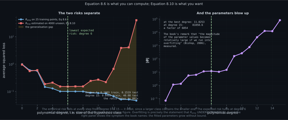
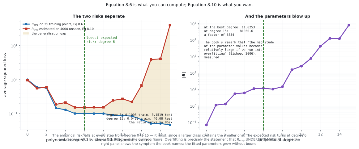
Reading the plot

The first figure is the section’s whole argument in two curves. The blue curve is $R_{\text{emp}}$, Equation 8.6 — the thing you can compute. It falls at every single step, from $0.993663$ at degree $0$ to $0.046494$ at degree $15$. There is no kink, no elbow, and no signal in its shape that says stop here.

The red curve is $R_{\text{true}}$, Equation 8.10 — estimated on $4000$ points the model never saw. It turns at degree $6$ with a value of $0.151857$, and then climbs to $40.077320$. The ratio between them reaches $862$. The shaded band is the generalisation gap, and the book’s definition of overfitting is exactly that the training risk underestimates the expected risk: measured here, the ratio exceeds $1$ from degree $2$ onward and never returns.

The right panel is worth pairing with the left because it shows the symptom rather than the disease. The book’s remark, citing Bishop (2006), is that “the magnitude of the parameter values becomes relatively large if we run into overfitting”. Measured: $\lVert\boldsymbol\theta\rVert$ goes from $11.8253$ at the best degree to $81{,}050.6$ at degree $15$ — a factor of $6854$. That is a signal you can compute from training data alone, and it is precisely what §8.2.3’s penalty term attacks.

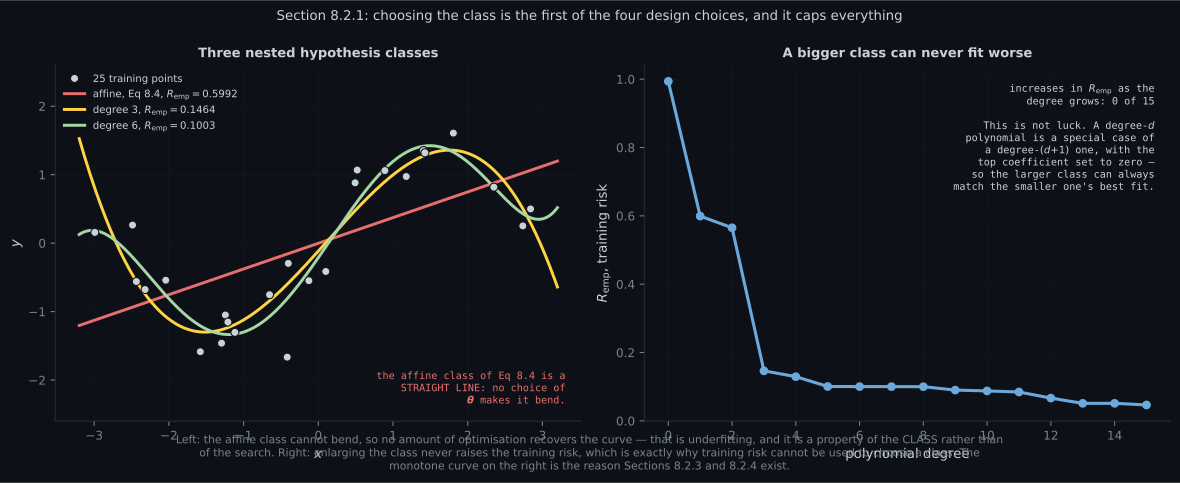
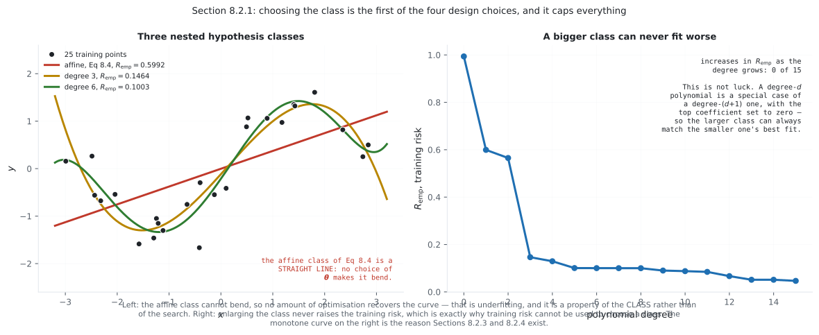
The second figure separates two kinds of failure. The left panel’s red line is the affine class of Equation 8.4, and its problem is not that the optimiser did badly — it is that no member of the class can bend. That is underfitting, and it is a property of the class you chose, not of the search you ran. More iterations, a better step size, a different initialisation: none of it helps.

The right panel is the fact that makes model selection necessary. Enlarging the class raised the training risk zero times in fifteen attempts, and that is not a property of this dataset. A degree-$d$ polynomial is a degree-$(d+1)$ polynomial with the top coefficient set to zero, so the larger class literally contains the smaller one’s best answer. Any criterion that only looks at training risk will always choose the largest class available. Given that, §8.2.3 and §8.2.4 are not refinements; they are the only things standing between you and degree $15$.

The third figure is the one people skip and shouldn’t. Predictor A is mediocre everywhere; predictor B is excellent almost everywhere and terrible occasionally. Which is better? The honest answer is it depends what you are going to do with it — and the three measures disagree.

Squared loss puts A ahead by $2.29\times$, because squaring turns twelve errors of $3.4$ into a large number. Absolute loss puts B ahead by $2.70\times$, because it counts A’s two hundred small errors at face value. The tolerance measure — does the prediction land within $1$? — scores A at exactly $0.0000$, a perfect record, because $0.55 < 1$.

So the same two predictors are ranked in two different orders by three reasonable measures. The book’s point is that the loss you optimise is chosen for optimisation convenience (squared loss is smooth and has a closed form; the tolerance measure has zero gradient almost everywhere), while the measure you are judged on comes from the application. When those differ, a training log full of falling squared loss tells you nothing about the number you will be evaluated on.

From the book

This page covers §8.2, §8.2.1 and §8.2.2 of Mathematics for Machine Learning by Deisenroth, Faisal and Ong (draft of 2019-12-11). The four design choices are listed at the head of §8.2. Equation 8.3 is the fitting goal, 8.4 and 8.5 are Example 8.1’s linear and affine forms. Equation 8.6 defines the empirical risk and the term empirical risk minimization; the i.i.d. assumption and its justification via §6.4.5 and §6.4.1 are the book’s. Example 8.2 gives the squared loss and Equations 8.7, 8.8 and 8.9, with the closed-form solution deferred to §9.2. Equation 8.10 is the expected risk, also called the population risk. The closing remark that the loss function and the performance measure often mismatch “due to issues such as ease of implementation or efficiency of optimization” is the book’s, as is the attribution of empirical risk minimization to the support vector machine and the Bishop (2006) remark about parameter magnitudes. The degree sweep, the $862\times$ ratio, the $6854\times$ parameter growth, and the three-measure reversal are this module’s additions.

Pitfalls

Choosing a model class by training risk

Measured: enlarging the class lowered the training risk at all fifteen steps and raised it at none. That is structural, since nested classes contain each other’s best answers — so any selection rule based on training risk alone will always pick the largest class on offer. At degree $15$ that means an expected risk $862\times$ the training figure.

Reading a low training risk as a good model

$R_{\text{emp}}$ at degree $15$ is $0.046494$, the best in the table. $R_{\text{true}}$ there is $40.077320$, the worst by a factor of $150$ over the next-worst. The two numbers are computed from the same predictor, and one of them is a fantasy.

Optimising a loss that is not your performance measure

Squared loss ranks predictor A above B; absolute loss ranks B above A, by comparable margins in opposite directions. If your report is graded on mean absolute error and your optimiser minimises squared error, every number in your training log can improve while the reported metric gets worse. The book flags this as common practice rather than an error, which makes it worth checking explicitly.

Forgetting that the i.i.d. assumption is doing work

Equation 8.6 averages the loss. The justification is that independence makes the empirical mean a good estimate of the population mean (§6.4.1). With time series, repeated measurements on the same subject, or data collected in batches, that assumption fails — and then the average training loss is not estimating what you think, before any question of overfitting arises.

Treating the empirical risk as a function of the predictor alone

The book writes $R_{\text{emp}}(f, \mathbf{X}, \mathbf{y})$ with three arguments deliberately. The same $f$ has a different empirical risk on different data, and §8.2.4’s cross-validation is entirely built on evaluating one $f$ against several different $\mathbf{X}, \mathbf{y}$. Notation that hides the data makes that step look like a trick.

Assuming a zero training risk means the model is right

With $N$ points, any polynomial of degree $N-1$ achieves exactly zero training risk on any data. In the worked example above the quadratic reaching zero happened to be correct, but a cubic would reach zero too. Interpolation and correctness are indistinguishable from the training risk.

Compare

	empirical risk, Eq 8.6	expected risk, Eq 8.10
what it averages over	your $N$ training points	the infinite population
computable	yes	no, ever
notation	$R_{\text{emp}}(f, \mathbf{X}, \mathbf{y})$	$R_{\text{true}}(f)$
depends on the data	yes, explicitly	no — the data is integrated out
behaviour as the class grows	never increases	turns
measured at degree 6	$0.100253$	$0.151857$
measured at degree 15	$0.046494$	$40.077320$
estimated by	—	a test set, or §8.2.4’s cross-validation

design choice	question	section
hypothesis class	what functions may $f$ be?	§8.2.1
loss function	how well does $f$ do on the training data?	§8.2.2
regularisation	how do we build predictors that generalise?	§8.2.3
search procedure	how do we explore the space of models?	§8.2.4

pch.quizTag Do you know which risk is which?

1. Why can the training risk never increase when you enlarge the hypothesis class?

   A Because the optimiser gets better with more parameters B Because a degree-d polynomial IS a degree-(d+1) one with the top coefficient zero, so the larger class contains the smaller one's best answer C It can increase; that is what overfitting means D Because the squared loss is convex
   pch.quizShowAnswer

   B — Because a degree-d polynomial IS a degree-(d+1) one with the top coefficient zero, so the larger class contains the smaller one's best answer — Nested classes contain each other's optima, so this is structural rather than empirical — measured, zero of fifteen steps raised the training risk. The consequence is the important part: any criterion based on training risk alone will always choose the largest class available.

2. What does the book define overfitting as, precisely?

   A A model with too many parameters B The training risk UNDERESTIMATING the expected risk for a given predictor C A training risk of zero D A model that fails on the validation set
   pch.quizShowAnswer

   B — The training risk UNDERESTIMATING the expected risk for a given predictor — The definition is a relation between two numbers for one fixed predictor, not a property of the parameter count. Measured on the sweep, the ratio exceeds one from degree 2 onward and reaches 862 by degree 15 — while the training risk kept falling.

3. Predictor A is off by 0.55 on all 200 points; B is exact on 188 and off by 3.4 on twelve. Which is better?

   A A, since squared loss gives 0.3025 against 0.6936 B B, since absolute loss gives 0.2040 against 0.5500 C It depends on the measure: squared and tolerance prefer A, absolute prefers B, and the ranking genuinely reverses D They are equivalent
   pch.quizShowAnswer

   C — It depends on the measure: squared and tolerance prefer A, absolute prefers B, and the ranking genuinely reverses — Three reasonable measures, two different winners. The book's remark is that the loss you optimise is usually chosen for optimisation convenience while the measure you are judged on comes from the application — so a training log of falling squared loss says nothing about a reported mean absolute error.

4. What role does the i.i.d. assumption play in Equation 8.6?

   A It makes the loss function convex B Independence makes the empirical mean a good estimate of the population mean, which is what licenses averaging the loss at all C It guarantees the model will generalise D It is needed only for the closed-form least-squares solution
   pch.quizShowAnswer

   B — Independence makes the empirical mean a good estimate of the population mean, which is what licenses averaging the loss at all — Section 8.2.2 gives exactly this justification, pointing at Sections 6.4.5 and 6.4.1. With time series or repeated measures the assumption fails and the average training loss is no longer estimating what you think — a problem that arrives before any question of overfitting.

5. You fit a degree-(N-1) polynomial to N points and get exactly zero training risk. What have you learned?

   A That the model is correct B Nothing: any degree-(N-1) polynomial interpolates any N points, so zero training risk is guaranteed regardless of the data C That the data is noise-free D That the hypothesis class is too small
   pch.quizShowAnswer

   B — Nothing: any degree-(N-1) polynomial interpolates any N points, so zero training risk is guaranteed regardless of the data — Interpolation and correctness are indistinguishable from the training risk. In the worked example the quadratic that reached zero happened to be right, but a cubic would also reach zero on the same four points — and the training risk cannot tell them apart.

🧪 Try It Yourself

Exercise 1 – Equation 8.9, two ways

pch.exerciseTag pch.exerciseTitle

Exercise 2 – The training risk never rises

pch.exerciseTag pch.exerciseTitle

Exercise 3 – The generalisation gap

pch.exerciseTag pch.exerciseTitle

Exercise 4 – The parameter norm is the symptom

pch.exerciseTag pch.exerciseTitle

Exercise 5 – Three measures, two winners

pch.exerciseTag pch.exerciseTitle

Recall card

• Four design choices, and the book numbers them: the hypothesis class (8.2.1), the loss function (8.2.2), regularisation (8.2.3), and the search procedure (8.2.4).
• Equation 8.6, the empirical risk, is the average loss over your N training points. Note it takes THREE arguments — the predictor and the data — because the same f scores differently on different data, which is what cross-validation exploits.
• The i.i.d. assumption is load-bearing. Independence is what makes the empirical mean a good estimate of the population mean, and therefore what licenses averaging the loss at all. Time series and repeated measures break it.
• Equation 8.10, the expected risk, is an expectation over the infinite population. It is what “good” means and it is never computable.
• Overfitting is defined as a relation between the two: the training risk UNDERESTIMATING the expected risk for a fixed predictor. It is not a statement about parameter counts.
• A bigger class can never fit the training data worse, because a degree-d polynomial is a degree-(d+1) one with a zero top coefficient. Measured: zero increases in fifteen steps. So training risk alone always endorses the largest class available.
• Measured sweep: training risk falls from 0.993663 to 0.046494 while the expected risk turns at degree 6 (0.151857) and reaches 40.077320 at degree 15 — a ratio of 862.
• The symptom you CAN compute is the parameter norm. It goes from 11.8253 at the best degree to 81050.6045 at degree 15, a factor of 6854 — which is the book’s Bishop (2006) remark, and exactly what Section 8.2.3 penalises.
• Underfitting is a property of the class, not the search. The affine class cannot bend; no step size or initialisation fixes that.
• Zero training risk proves nothing. Any degree-(N-1) polynomial interpolates any N points, so interpolation and correctness are indistinguishable from the training risk.
• The loss you optimise is not the measure you are judged on. Measured: predictor A beats B on squared loss (0.3025 to 0.6936) and loses on absolute loss (0.5500 to 0.2040). The ranking reverses, and the book notes the mismatch is usual rather than exceptional.
• Example 8.2’s least-squares problem has a closed form, via the normal equations of Section 9.2 — one of the few places in the chapter where the optimisation is free.

Next: the two repairs — bias the search, and estimate the risk you cannot compute. Regularization and Cross-Validation