Attention from Scratch (Queries, Keys and Values)

Recurrence reads a sequence one step at a time and carries a state. Phase 4 measured what that costs: a SimpleRNN stopped working between 40 and 100 timesteps, and even an LSTM failed at 200.

Attention takes the opposite approach. Every position looks at every other position directly, in one step, with weights that depend on content. There is no state to decay, and the path between any two positions has length 1.

$$\mathrm{Attention}(Q, K, V) = \mathrm{softmax}\!\left(\frac{QK^\top}{\sqrt{d_k}}\right)V$$

That is the whole operation. This page implements it in six lines of NumPy, checks it against keras.layers.MultiHeadAttention (agreeing to 2.03e-07), measures why the $\sqrt{d_k}$ is there, and then finds a task that a single attention layer cannot solve no matter how long you train it.

What you’ll learn

• Queries, keys and values as a lookup: what each one is for, not just its shape.
• The measured reason for the scale factor: without it, the largest attention weight climbs from 0.4442 at $d_k = 4$ to 0.9355 at $d_k = 256$.
• Causal and padding masks, and what each one blocks.
• Multi-head attention as several lookups in parallel.
• A task where one attention block scores 0.3120 and two score 0.9990 — and the circuit that makes the difference.

Queries, keys and values

The names come from dictionary lookup. In a Python dict you compare a key for equality and get back exactly one value. Attention softens both halves: it compares a query against every key by dot product, turns those scores into weights that sum to 1, and returns the weighted average of the values.

Scaled dot-product attention, in full

def attention(query, key, value, mask=None):
    scores = query @ key.T                       # (queries, keys) similarity
    scores = scores / np.sqrt(query.shape[-1])   # the scale — see below
    if mask is not None:
        scores = np.where(mask, scores, -1e9)    # blocked pairs get -inf
    weights = softmax(scores, axis=-1)           # each row sums to 1
    return weights @ value, weights

Three separate projections turn one sequence into $Q$, $K$ and $V$ — which is what makes the operation learnable. Self-attention is the case where all three come from the same tokens: every position asks its own question about every other position.

Run that NumPy against Keras with the layer’s own weights and the outputs differ by 2.03e-07, the attention weights by 6.48e-08. Float32 rounding, nothing else.

Why divide by $\sqrt{d_k}$

The dot product of two $d$-dimensional vectors with unit-variance components has variance $d$. Feed larger scores to a softmax and it saturates — all the weight lands on one key.

figure 200 random query-key draws, 12 tokens matplotlib

Without the scale, attention at d_k = 256 puts 0.9355 of its weight on a single token before any training — the softmax has saturated on noise, and its gradient with it. The scaled version holds near 0.28 at every dimension, which is the point: the operation should behave the same whether the head is 4-dimensional or 256-dimensional. The entropy panel says the same thing in nats, against a uniform maximum of 2.4849.

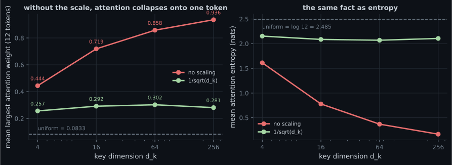
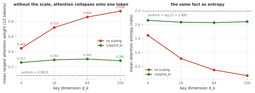
$d_k$	Max weight, unscaled	Max weight, scaled	Entropy, unscaled	Entropy, scaled
4	0.4442	0.2567	1.6128	2.1533
16	0.7189	0.2918	0.7792	2.0866
64	0.8577	0.3024	0.3698	2.0702
256	0.9355	0.2812	0.1668	2.1064

Uniform attention over 12 tokens is 0.0833 with entropy $\log 12 = 2.4849$. A saturated softmax is not just badly behaved at the forward pass — its gradient is near zero everywhere except at the winning key, so the layer stops learning which key it should have picked.

Masks

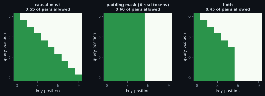
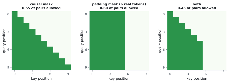
A mask is applied to the scores, before the softmax, by setting blocked pairs to a large negative number. After the softmax they hold exactly zero weight — measured 0.00e+00, not “approximately zero”.

figure Causal, padding, and both matplotlib

The causal mask stops a position seeing the future, which is what makes a decoder trainable in parallel: every position predicts its next token at once, and none of them can cheat. The padding mask stops every position attending to positions that are not really there — the attention-shaped version of the same bug measured in Phase 4, where post-padding without a mask dropped a SimpleRNN to chance.

Mask	Pairs allowed
causal (10 positions)	0.5500
padding (6 of 10 real)	0.6000
both	0.4500

The two are not interchangeable. Causal masking is about what the model is allowed to know; padding masking is about what actually exists. A decoder needs both.

Multi-head attention

One head produces one weighted average. If a position needs both “the noun this adjective modifies” and “the last time this token appeared”, one softmax cannot deliver both — its weights sum to 1 and must be spent somewhere.

h heads, each of width d_model / h

attention = keras.layers.MultiHeadAttention(num_heads=4, key_dim=64 // 4)
output = attention(tokens, tokens)                        # self-attention
output, scores = attention(tokens, tokens, return_attention_scores=True)

Splitting a 64-dimensional model into 4 heads of 16 costs no extra parameters — the same projection matrices are reshaped — and buys four independent lookups.

A task one attention layer cannot do

Here is the sharpest measurement on the page. The task: a sequence of symbols contains a cue symbol exactly once; the same cue is repeated at the final position as a query; the answer is the token that came immediately after the earlier cue.

text

symbols:  3 7 2 [CUE] 5 1 4 6 2 ... [CUE]
                       ^ the answer is 5

Attention blocks	Parameters	Best validation accuracy
1	9,129	0.3120
2	17,673	0.9990

Chance is 0.1429. One block gets barely above it; two blocks solve it essentially perfectly. Nothing else changed — same data, same seed, same 30 epochs.

figure Match the cue, then read the next token matplotlib

The left panel is a capability boundary, not a tuning difference — the one-block model never improves. The right panel shows the circuit the two-block model found: the second block's query attends almost entirely to offset -1, which is the cue position rather than the answer position. The first block has already let each position absorb its neighbour, so by the time the second block matches the cue, the cue position is carrying the answer.

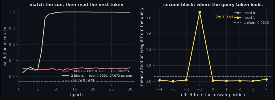
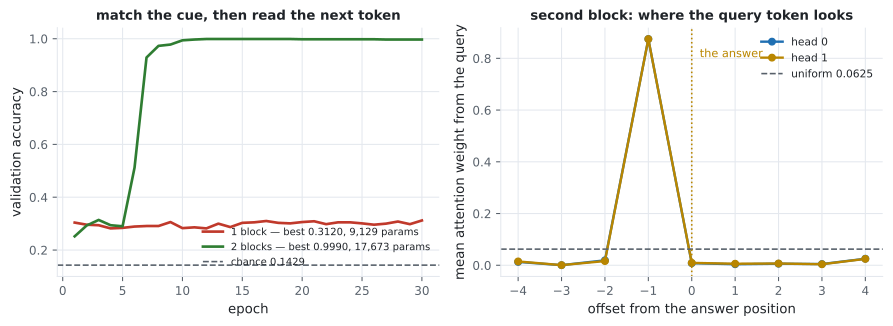
Why one layer is not enough. Solving the task requires two operations: match the query against the cue by content, and move one position along. A single attention layer does one weighted average — it can match content or apply a fixed positional offset, but not compose them. Two layers can, and the measured attention shows exactly how: the first block moves neighbour information into each position, the second block matches the cue and reads what is now there.

This composition has a name in the interpretability literature — an induction head — and it is the smallest example of why depth buys qualitatively new behaviour rather than just capacity. It also explains the shape of the learning curve: the two-block model sits at chance for five epochs and then jumps to 1.00 in three, because the circuit only works once both halves exist.

diagram Diagram mermaid

  flowchart LR
  A["query: the cue symbol
at the last position"] --> B["block 1
every position absorbs
its neighbour"]
  B --> C["block 2
match the query
against the cue"]
  C --> D["read the cue position
— it now holds the answer"]
  E["one block only"] --> F["can match OR shift,
not both — 0.3120"]

sketch Attention as a soft lookup p5.js Pause Restart

Drag the query vector. The bars are the attention weights over five keys; the output is their weighted average of the values.

sketch The measured table, ranked p5.js Pause Restart

Click a column to rank every row by it. The bars are that column's values and the highest and lowest are computed from the numbers, not written in.

Pitfalls

• Dropping the $1/\sqrt{d_k}$. At $d_k = 256$ the largest weight is 0.9355 before training: a saturated softmax with almost no gradient.
• Masking after the softmax. The weights no longer sum to 1. Mask the scores, then normalise.
• Using a large negative constant instead of -inf carelessly. -1e9 is fine in float32; -1e30 overflows to -inf in float16 and produces NaN when a whole row is masked.
• Forgetting the padding mask. Attention will happily average padding vectors, which is the same class of bug that dropped a SimpleRNN to 0.5036 in Phase 4.
• Confusing causal with padding masks. One hides the future, the other hides what does not exist. A decoder needs both.
• Expecting one attention layer to compose two operations. Match-then-shift needed two blocks: 0.3120 against 0.9990.
• Reading attention weights as explanations. The head that solved this task put 0.87 on the cue position — but on Vision Transformers a confidently wrong prediction had entirely unremarkable attention.

Recap

• Attention is softmax(QKᵀ/√d_k)V — a soft dictionary lookup returning a weighted average of values. Six lines, matching Keras to 2.03e-07.
• The scale exists because dot-product variance grows with $d_k$: unscaled max weight 0.4442 → 0.9355 as $d_k$ goes 4 → 256, entropy 1.6128 → 0.1668.
• Masks are applied to the scores before the softmax and leave exactly 0.00e+00 weight.
• Causal masks allowed 0.5500 of pairs, padding masks 0.6000, both 0.4500.
• Multiple heads cost no extra parameters and buy independent lookups.
• One attention block scored 0.3120 on match-then-read; two scored 0.9990. Depth composes operations that width cannot.

Next

Attention plus a feed-forward block, residuals and normalisation is a transformer. The full architecture, measured against the recurrent models from Phase 4: The Transformer Architecture.

pch.quizTag pch.quizDefaultTitle

1. Why is the attention score divided by the square root of the key dimension?

   A To keep the output in the range [0, 1] B Because the dot product of d-dimensional vectors has variance d, so without the scale the softmax saturates — measured 0.9355 of the weight on one token at d_k = 256, before any training C To make the gradients larger D Because the softmax requires normalised inputs
   pch.quizShowAnswer

   B — Because the dot product of d-dimensional vectors has variance d, so without the scale the softmax saturates — measured 0.9355 of the weight on one token at d_k = 256, before any training — A saturated softmax also has a near-zero gradient, so the layer stops learning which key it should have chosen.

2. A causal mask on 10 positions allows 0.5500 of query-key pairs, and a padding mask with 6 real tokens allows 0.6000. What is the difference in purpose?

   A They are two names for the same thing B The causal mask hides the future — what the model is allowed to know; the padding mask hides positions that do not exist. A decoder needs both C The causal mask is applied after the softmax D Padding masks are only needed for images
   pch.quizShowAnswer

   B — The causal mask hides the future — what the model is allowed to know; the padding mask hides positions that do not exist. A decoder needs both — Combining both left 0.4500 of pairs allowed. Omitting the padding mask is the attention-shaped version of the post-padding bug from Phase 4.

3. One attention block scored 0.3120 on the match-then-read task; two blocks scored 0.9990. What does that show?

   A The one-block model needed more epochs B A capability boundary — one weighted average can match content or shift position, not compose both; the second block is what turns a match into a lookup C Two blocks simply have more parameters D The task is impossible without recurrence
   pch.quizShowAnswer

   B — A capability boundary — one weighted average can match content or shift position, not compose both; the second block is what turns a match into a lookup — The one-block curve is flat for all 30 epochs. The two-block model sits at chance for five epochs then jumps to 1.00, because the circuit only works once both halves exist.

4. The trained second block put about 0.87 of its attention on offset -1 — the cue position, not the answer position. Why?

   A The measurement is off by one B The first block already moved each position's neighbour into it, so by the time the second block matches the cue, the cue position is carrying the answer C Attention cannot address the correct position D The model memorised the training set
   pch.quizShowAnswer

   B — The first block already moved each position's neighbour into it, so by the time the second block matches the cue, the cue position is carrying the answer — This is the induction-head circuit: a previous-token step followed by a matching step. It is why the behaviour appears suddenly rather than gradually.

5. What does splitting a 64-dimensional attention layer into 4 heads of 16 cost?

   A Four times the parameters B No extra parameters — the same projection matrices are reshaped — in exchange for four independent lookups instead of one weighted average C Four times the memory but the same compute D It requires four times the training data
   pch.quizShowAnswer

   B — No extra parameters — the same projection matrices are reshaped — in exchange for four independent lookups instead of one weighted average — One softmax's weights sum to 1, so a single head cannot attend to two things at once. Heads are how a layer asks several questions in parallel.

🧪 Try It Yourself

pch.exerciseTag pch.exerciseTitle

pch.exerciseTag pch.exerciseTitle

pch.exerciseTag pch.exerciseTitle

pch.exerciseTag pch.exerciseTitle

pch.exerciseTag pch.exerciseTitle