Problem Formulation

Chapter 8 built a vocabulary. Chapter 9 spends it on one problem — and does so three times, once per flavour of learning: maximum likelihood (§9.2.1), MAP (§9.2.3), and full Bayesian inference (§9.3).

This page is the setup all three share. It looks like bookkeeping. Two of its choices are not.

What you’ll learn

• Equation 9.1: why the chapter starts with a likelihood rather than a loss.
• Equations 9.3 and 9.4 — and the restriction their caption states in passing: straight lines through the origin. Measured, that costs RMSE $4.091288$ against $0.514303$ on data with an intercept, and gets the slope wrong too.
• Equation 9.5’s factorization, and the conditional independence in Figure 9.3 that licenses it — verified to $1.4\times10^{-15}$.
• Why the log-transform is not cosmetic: measured, the product of $N$ densities is exactly $0.0$ in float64 by $N = 1000$.
• “Linear regression refers to models that are linear in the parameters.” Measured: superposition holds in $\boldsymbol\theta$ to $4.4\times10^{-11}$ and fails in $x$ by $2.3\times10^{5}$.
• The remark that the likelihood “does not integrate to 1” in $\boldsymbol\theta$ — measured, it integrates to exactly $1/\lvert x\rvert$.
• Equation 9.6’s predictive, whose width is $\sigma$ everywhere — the plug-in interval page 806 measured at $0.1796$ coverage.

Intuition: two nouns doing different jobs

$p(y \mid x, \boldsymbol\theta) = \mathcal{N}(y \mid x^\top\boldsymbol\theta, \sigma^2)$ is one formula and two objects.

Slide $y$ and hold everything else. You get a bell curve over possible observations. It integrates to one. It is a probability density, and it says: given these parameters and this input, here is how the measurement will scatter.

Slide $\boldsymbol\theta$ and hold everything else. You get a curve that looks the same and is not a density. It does not integrate to one — measured below, it integrates to $1/\lvert x\rvert$. It is the likelihood, and it says: given what I actually saw, here is how well each parameter explains it.

Maximum likelihood maximises the second while calling it a probability. That abuse is harmless — the argmax is unaffected — right up until §9.2.3 wants to divide by something, at which point the missing normaliser becomes the marginal likelihood and the whole of §9.3.5.

diagram One formula, and where each reading leads mermaid

  flowchart TD
  L["p(y | x, theta) = N(y | x'theta, sigma^2)
Equation 9.1"]
  L -->|"vary y, fix theta"| D["a DENSITY over data
integrates to 1.00000000"]
  L -->|"vary theta, fix y"| K["the LIKELIHOOD
integrates to 1/|x| = 0.5"]
  D --> P["Eq 9.6: the predictive
width sigma, everywhere"]
  K --> ML["9.2.1 maximise it
= least squares"]
  K --> MAP["9.2.3 multiply by a prior
= regularised least squares"]
  K --> BAY["9.3 normalise it properly
= a posterior, and 9.3.5's integral"]

§9.1 Problem formulation

Because of “the presence of observation noise”, the chapter adopts a probabilistic approach and models the noise explicitly:

$$p(y \mid x) = \mathcal{N}\!\left(y \mid f(x), \sigma^2\right) \qquad \text{(9.1)}$$

with $x \in \mathbb{R}^D$ the inputs and $y \in \mathbb{R}$ the “noisy function values (targets)”. Equivalently,

$$y = f(x) + \epsilon, \qquad \epsilon \sim \mathcal{N}(0, \sigma^2) \qquad \text{(9.2)}$$

with $\epsilon$ i.i.d. Gaussian measurement noise. The objective: “to find a function that is close (similar) to the unknown function $f$ that generated the data and that generalizes well.”

Two standing assumptions for most of the chapter: the model is parametric, and $\sigma^2$ is known. (§9.2.1 relaxes the second at the end, with Equation 9.22.)

The linear case

$$p(y \mid x, \boldsymbol\theta) = \mathcal{N}\!\left(y \mid x^\top\boldsymbol\theta, \sigma^2\right) \quad\Longleftrightarrow\quad y = x^\top\boldsymbol\theta + \epsilon \qquad \text{(9.3), (9.4)}$$

Read the sentence after Equation 9.4

The class of functions described by (9.4) are straight lines that pass through the origin.

There is no intercept. Not “the intercept is omitted for clarity” — the model as written cannot produce one. Measured on data that really is $y = 4.0 + 1.3x + \epsilon$:

model	parameters found	RMSE	prediction at $x = 0$
Eq 9.4, $f(x) = x\theta$	$\theta = 1.193712$	$\mathbf{4.091288}$	$0.000000$ (forced)
Eq 9.13, $\phi(x) = [1, x]^\top$	$[4.077706, 1.329905]$	$\mathbf{0.514303}$	$4.077706$

The damage is not confined to the intercept. The one-parameter model’s slope comes out at $1.193712$ against a true $1.3$ — wrong by $0.106288$ — because it is spending its single parameter trying to reach a data cloud whose centre is not at the origin. A missing feature corrupts the features you kept.

§9.1 also notes “we chose a parametrization $f(x) = x^\top\boldsymbol\theta$” — chose. Equation 9.13 chooses differently and nothing else in the chapter changes.

Where the uncertainty comes from, and the Dirac limit

“The only source of uncertainty originates from the observation noise (as $x$ and $\boldsymbol\theta$ are assumed known in (9.3)).” Without it, “the relationship between $x$ and $y$ would be deterministic and (9.3) would be a Dirac delta” — the book’s margin note calling a delta “a Gaussian in the limit of $\sigma^2 \to 0$”.

Measured:

$\sigma^2$	peak height	area	mass within $\pm 0.01$
$10^{0}$	$0.3989$	$0.99993666$	$0.007978$
$10^{-2}$	$3.9894$	$1.00000000$	$0.079652$
$10^{-4}$	$39.8942$	$1.00000000$	$0.682665$
$10^{-6}$	$398.9423$	$1.00000000$	$1.000000$

The peak diverges, the area stays $1$, and the mass collapses onto a point.

Linear in the parameters

The chapter’s most load-bearing sentence, and it appears three times in the margin:

“Linear regression” refers to models that are “linear in the parameters”, i.e., models that describe a function by a linear combination of input features. Here, a “feature” is a representation $\phi(x)$ of the inputs $x$.

Superposition, measured both ways

For a degree-9 model with $\phi(x) = [1, x, x^2, \ldots, x^9]^\top$:

$$\max\left\lvert f(x;\ a\boldsymbol\theta_1 + b\boldsymbol\theta_2) - a\,f(x;\boldsymbol\theta_1) - b\,f(x;\boldsymbol\theta_2)\right\rvert = 4.366\times10^{-11}$$$$\max\left\lvert \phi(a u + b v) - a\,\phi(u) - b\,\phi(v)\right\rvert = 2.341\times10^{5}$$

Linear in $\boldsymbol\theta$ to floating-point; violently nonlinear in $x$. A degree-9 polynomial fit is an ordinary linear least-squares solve — which is why Equation 9.19 will be Equation 9.12c with $\mathbf{X}$ replaced by $\boldsymbol\Phi$, and nothing else.

§9.2 Parameter estimation

Given a training set $\mathcal{D} := \{(x_1, y_1), \ldots, (x_N, y_N)\}$, Figure 9.3’s graphical model (page 807’s notation: shaded nodes are observed, deterministic values lose their circle) shows $\boldsymbol\theta$ and $\sigma$ outside a plate over $n = 1, \ldots, N$, with $x_n$ and $y_n$ inside.

”$y_i$ and $y_j$ are conditionally independent given their respective inputs $x_i, x_j$”, so the likelihood factorizes:

$$p(\mathcal{Y} \mid \mathcal{X}, \boldsymbol\theta) = \prod_{n=1}^{N} p(y_n \mid x_n, \boldsymbol\theta) = \prod_{n=1}^{N}\mathcal{N}\!\left(y_n \mid x_n^\top\boldsymbol\theta, \sigma^2\right) \qquad \text{(9.5)}$$

Equation 9.5, checked

On $N = 12$ points, the joint as a single $12$-dimensional Gaussian with covariance $\sigma^2\mathbf{I}$ against the product of $12$ scalar Gaussians:

	value
$p(\mathcal{Y} \mid \mathcal{X}, \boldsymbol\theta)$, one $12$-d Gaussian	$6.199453\times10^{-4}$
$\prod_n p(y_n \mid x_n, \boldsymbol\theta)$, $12$ factors	$6.199453\times10^{-4}$
relative difference	$1.399\times10^{-15}$

The plate is not a drawing convention — it is this equality, exactly as page 807 measured for the Bernoulli case.

Once $\boldsymbol\theta^*$ is found, the prediction at a test input $x_*$ is

$$p(y_* \mid x_*, \boldsymbol\theta^*) = \mathcal{N}\!\left(y_* \mid x_*^\top\boldsymbol\theta^*, \sigma^2\right) \qquad \text{(9.6)}$$

Equation 9.6’s width does not depend on where you ask

$x_*$	mean	predictive sd	95% width
$0.0$	$4.077706$	$0.600000$	$2.351957$
$5.0$	$10.727230$	$0.600000$	$2.351957$
$100.0$	$137.068186$	$0.600000$	$2.351957$

Constant, forever. Equation 9.6 substitutes a point estimate into the likelihood, so the only uncertainty left is the observation noise. This is exactly the plug-in predictive page 806 measured at $\mathbf{0.1796}$ coverage in extrapolation while labelled $95\%$. §9.3 is the chapter’s answer, and Equation 9.6 is what it replaces.

The likelihood is not a distribution over parameters

§9.2.1’s remark:

The likelihood $p(y \mid x, \boldsymbol\theta)$ is not a probability distribution in $\boldsymbol\theta$: It is simply a function of the parameters $\boldsymbol\theta$ but does not integrate to 1 (i.e., it is unnormalized), and may not even be integrable with respect to $\boldsymbol\theta$. However, the likelihood in (9.7) is a normalized probability distribution in $y$.

Measured — and the answer is exact

For $p(y \mid x, \theta) = \mathcal{N}(y \mid x\theta, \sigma^2)$ with $x = 2$, $\sigma = 0.6$:

integral	value
$\int p(y \mid x{=}2, \theta{=}1.3)\,dy$	$\mathbf{1.00000000}$
$\int p(y{=}3.1 \mid x{=}2, \theta)\,d\theta$	$\mathbf{0.50000000}$

The second is exactly $1/\lvert x\rvert$. Substituting $u = x\theta$ gives $d\theta = du/\lvert x\rvert$, so the integral is $1/\lvert x\rvert$ for every $x \neq 0$.

So it reaches $1$ only by accident when $\lvert x\rvert = 1$, and diverges as $x \to 0$ — the book’s “may not even be integrable”, made concrete.

Why the log-transform

The book gives two reasons: “(a) it does not suffer from numerical underflow, and (b) the differentiation rules will turn out simpler”, since “we cannot represent very small numbers, such as $10^{-256}$”, and the log turns a product into a sum “such that the corresponding gradient is a sum of individual gradients, instead of a repeated application of the product rule (5.46)”.

Reason (a), measured — this is not a stylistic preference

$N$	$\prod_n p(y_n \mid x_n, \boldsymbol\theta)$	$\sum_n \log p(y_n \mid x_n, \boldsymbol\theta)$
$10$	$2.953338\times10^{-4}$	$-8.127404$
$100$	$5.767475\times10^{-37}$	$-83.443414$
$300$	$9.500084\times10^{-117}$	$-267.151155$
$700$	$1.481966\times10^{-275}$	$-632.817531$
$1000$	$\mathbf{0.000000\times10^{0}}$	$-898.461655$
$5000$	$\mathbf{0.000000\times10^{0}}$	$-4614.434798$

By $N = 1000$ the product is exactly zero in float64 — and a gradient of zero is not a small gradient, it is no gradient. The sum is an ordinary number at every $N$. The smallest positive float64 is $4.940656\times10^{-324}$, and $1000$ typical densities multiply straight past it.

Worked example by hand

Fit $f(x) = \theta x$ — Equation 9.4 with $D = 1$ — to three points, from the likelihood.

Data: $(1, 2.1)$, $(2, 3.8)$, $(3, 6.3)$, with $\sigma^2$ known.

Step 1: write the likelihood. By Equation 9.5,

$$p(\mathcal{Y} \mid \mathcal{X}, \theta) = \prod_{n=1}^{3}\frac{1}{\sqrt{2\pi\sigma^2}}\exp\!\left(-\frac{(y_n - x_n\theta)^2}{2\sigma^2}\right)$$

Step 2: take the negative log. The product becomes a sum, and every $\theta$-free term becomes a constant:

$$\mathcal{L}(\theta) = \frac{1}{2\sigma^2}\sum_{n=1}^{3}(y_n - x_n\theta)^2 + \text{const}$$

Step 3: differentiate and set to zero. $\sigma^2 > 0$ is a positive constant, so it cannot move the minimiser:

$$\frac{d\mathcal{L}}{d\theta} = -\frac{1}{\sigma^2}\sum_n x_n(y_n - x_n\theta) = 0 \quad\Longrightarrow\quad \theta\sum_n x_n^2 = \sum_n x_n y_n$$

Step 4: solve.

$$\sum_n x_n^2 = 1 + 4 + 9 = 14, \qquad \sum_n x_n y_n = 2.1 + 7.6 + 18.9 = 28.6$$ $$\boxed{\ \theta_{\text{ML}} = \frac{28.6}{14} = 2.042857\ }$$

Step 5: recognise it. $\theta = \dfrac{\sum x_n y_n}{\sum x_n^2} = \dfrac{\mathbf{x}^\top\mathbf{y}}{\mathbf{x}^\top\mathbf{x}}$ — which is Equation 9.12c, $(\mathbf{X}^\top\mathbf{X})^{-1}\mathbf{X}^\top\mathbf{y}$, in one dimension. It is also the projection coefficient of $\mathbf{y}$ onto $\mathbf{x}$ from §3.8. §9.4 makes that second reading the whole point.

Step 6: notice what $\sigma^2$ did. Nothing. It scaled the objective and vanished at the differentiation. That is why §9.2.2 can “ignore the scaling by $1/\sigma^2$” and work with $\lVert\mathbf{y} - \boldsymbol\Phi\boldsymbol\theta\rVert^2$ — and why $\sigma^2$ only becomes a real parameter when Equation 9.22 estimates it too.

See it move

sketch Two readings of one formula p5.js Pause Restart

The Gaussian likelihood of Equation 9.1, drawn as a function of y and as a function of theta. Drag x and watch the theta-reading stretch and squash while its area changes as one over the absolute value of x — and the y-reading keep an area of exactly one no matter what.

From scratch

problem_formulation.py

import numpy as np
 
# --- Equation 9.4 has no intercept --------------------------------------
rng = np.random.default_rng(11)
SIG = 0.6
TRUE_B, TRUE_A = 1.3, 4.0      # y = 4.0 + 1.3 x + noise
x = np.sort(rng.uniform(-5, 5, 40))
y = TRUE_A + TRUE_B * x + SIG * rng.standard_normal(40)
 
th_origin = float(x @ y / (x @ x))              # Eq 9.4, one parameter
Phi = np.column_stack([np.ones_like(x), x])     # Eq 9.13, phi = [1, x]
th_feat = np.linalg.lstsq(Phi, y, rcond=None)[0]
 
def rmse(pred):
    return float(np.sqrt(np.mean((y - pred) ** 2)))
 
print("=== 1. Equation 9.4: lines THROUGH THE ORIGIN ===")
print(f"the data really is y = {TRUE_A} + {TRUE_B} x + noise, sigma = {SIG}")
print(f"Eq 9.4   f(x) = x*theta : theta = {th_origin:.6f}   "
      f"RMSE {rmse(th_origin*x):.6f}")
print(f"Eq 9.13  phi = [1, x]   : theta = {np.round(th_feat,6).tolist()}  "
      f"RMSE {rmse(Phi @ th_feat):.6f}")
print(f"the slope alone is off by {abs(th_origin-TRUE_B):.6f}")
print(f"prediction at x = 0: 0.000000 (forced) vs {th_feat[0]:.6f}")
 
# --- Equation 9.5: the likelihood factorizes ----------------------------
print("\n=== 2. Equation 9.5: the likelihood factorizes ===")
N = 12
xs = rng.uniform(-5, 5, N)
th = np.array([4.0, 1.3])
P = np.column_stack([np.ones_like(xs), xs])
ys = P @ th + SIG * rng.standard_normal(N)
r = ys - P @ th
n = len(ys)
joint = float(np.exp(-0.5 * (r @ r) / SIG**2) / ((2*np.pi*SIG**2) ** (n/2)))
prod = float(np.prod(np.exp(-0.5*(r/SIG)**2) / (SIG*np.sqrt(2*np.pi))))
print(f"as one {n}-dimensional Gaussian : {joint:.6e}")
print(f"as {n} separate factors         : {prod:.6e}")
print(f"relative difference: {abs(joint-prod)/prod:.3e}")
 
# --- why the log-transform ----------------------------------------------
print("\n=== 3. the log-transform is not cosmetic: underflow ===")
print(f"{'N':>8} {'prod of densities':>20} {'sum of log densities':>22}")
rr = np.random.default_rng(5)
for Nn in (10, 100, 300, 700, 1000, 5000):
    res = SIG * rr.standard_normal(Nn)
    dens = np.exp(-0.5*(res/SIG)**2) / (SIG*np.sqrt(2*np.pi))
    print(f"{Nn:>8} {float(np.prod(dens)):>20.6e} "
          f"{float(np.sum(np.log(dens))):>22.6f}")
print(f"smallest positive float64 (subnormal): {np.nextafter(0, 1):.6e}")
 
# --- linear in the PARAMETERS -------------------------------------------
print("\n=== 4. 'linear regression' means linear in the PARAMETERS ===")
def phi(v, K=10):
    return np.vander(np.asarray(v, float), K, increasing=True)
xg = np.linspace(-4, 4, 9)
A = phi(xg)
r1 = np.random.default_rng(2)
t1, t2 = r1.standard_normal(10), r1.standard_normal(10)
a, b = 2.7, -1.4
print("superposition in theta, max |f(a t1 + b t2) - a f(t1) - b f(t2)|:")
print(f"  {np.abs(A @ (a*t1 + b*t2) - (a*(A @ t1) + b*(A @ t2))).max():.3e}"
      f"   -> LINEAR in theta")
u, v = 1.1, -0.7
print("superposition in x, max |phi(a u + b v) - a phi(u) - b phi(v)|:")
print(f"  {np.abs(phi(np.array([a*u + b*v]))[0] - (a*phi(np.array([u]))[0] + b*phi(np.array([v]))[0])).max():.3e}"
      f"   -> NOT linear in x")
 
# --- Equation 9.6's width does not depend on x --------------------------
print("\n=== 5. Equation 9.6: the predictive width is constant ===")
print(f"{'x*':>8} {'mean':>14} {'predictive sd':>15} {'95% width':>11}")
for xstar in (0.0, 2.0, 5.0, 20.0, 100.0):
    m = float(np.array([1.0, xstar]) @ th_feat)
    print(f"{xstar:>8.1f} {m:>14.6f} {SIG:>15.6f} "
          f"{2*1.959963984540054*SIG:>11.6f}")
 
# --- a density in y, NOT in theta ---------------------------------------
print("\n=== 6. the likelihood is a density in y, NOT in theta ===")
xq, sq, tq, yq = 2.0, 0.6, 1.3, 3.1
gy = np.linspace(-30, 30, 4_000_001)
dy = np.exp(-0.5*((gy - xq*tq)/sq)**2)/(sq*np.sqrt(2*np.pi))
print(f"integral over y of p(y | x={xq}, theta={tq}): "
      f"{np.trapezoid(dy, gy):.8f}")
gt = np.linspace(-60, 60, 4_000_001)
dt = np.exp(-0.5*((yq - xq*gt)/sq)**2)/(sq*np.sqrt(2*np.pi))
print(f"integral over theta of p(y={yq} | x={xq}, theta):  "
      f"{np.trapezoid(dt, gt):.8f}")
print(f"  it equals 1/|x| = {1/abs(xq):.6f}, so it reaches 1 only when")
print("  |x| = 1, and diverges as x -> 0")
 
# --- the Dirac limit -----------------------------------------------------
print("\n=== 7. without noise, Eq 9.3 becomes a Dirac delta ===")
print(f"{'sigma^2':>10} {'peak height':>14} {'area':>12} "
      f"{'mass within 0.01':>18}")
g = np.linspace(-4, 4, 8_000_001)
for s2 in (1.0, 1e-1, 1e-2, 1e-4, 1e-6):
    s = np.sqrt(s2)
    d = np.exp(-0.5*(g/s)**2)/(s*np.sqrt(2*np.pi))
    band = np.abs(g) <= 0.01
    print(f"{s2:>10.0e} {d.max():>14.4f} {np.trapezoid(d, g):>12.8f} "
          f"{np.trapezoid(d[band], g[band]):>18.6f}")

text

=== 1. Equation 9.4: lines THROUGH THE ORIGIN ===
the data really is y = 4.0 + 1.3 x + noise, sigma = 0.6
Eq 9.4   f(x) = x*theta : theta = 1.193712   RMSE 4.091288
Eq 9.13  phi = [1, x]   : theta = [4.077706, 1.329905]  RMSE 0.514303
the slope alone is off by 0.106288
prediction at x = 0: 0.000000 (forced) vs 4.077706
 
=== 2. Equation 9.5: the likelihood factorizes ===
as one 12-dimensional Gaussian : 6.199453e-04
as 12 separate factors         : 6.199453e-04
relative difference: 1.399e-15
 
=== 3. the log-transform is not cosmetic: underflow ===
       N    prod of densities   sum of log densities
      10         2.953338e-04              -8.127404
     100         5.767475e-37             -83.443414
     300        9.500084e-117            -267.151155
     700        1.481966e-275            -632.817531
    1000         0.000000e+00            -898.461655
    5000         0.000000e+00           -4614.434798
smallest positive float64 (subnormal): 4.940656e-324
 
=== 4. 'linear regression' means linear in the PARAMETERS ===
superposition in theta, max |f(a t1 + b t2) - a f(t1) - b f(t2)|:
  4.366e-11   -> LINEAR in theta
superposition in x, max |phi(a u + b v) - a phi(u) - b phi(v)|:
  2.341e+05   -> NOT linear in x
 
=== 5. Equation 9.6: the predictive width is constant ===
      x*           mean   predictive sd   95% width
     0.0       4.077706        0.600000    2.351957
     2.0       6.737515        0.600000    2.351957
     5.0      10.727230        0.600000    2.351957
    20.0      30.675802        0.600000    2.351957
   100.0     137.068186        0.600000    2.351957
 
=== 6. the likelihood is a density in y, NOT in theta ===
integral over y of p(y | x=2.0, theta=1.3): 1.00000000
integral over theta of p(y=3.1 | x=2.0, theta):  0.50000000
  it equals 1/|x| = 0.500000, so it reaches 1 only when
  |x| = 1, and diverges as x -> 0
 
=== 7. without noise, Eq 9.3 becomes a Dirac delta ===
   sigma^2    peak height         area   mass within 0.01
     1e+00         0.3989   0.99993666           0.007978
     1e-01         1.2616   1.00000000           0.025226
     1e-02         3.9894   1.00000000           0.079652
     1e-04        39.8942   1.00000000           0.682665
     1e-06       398.9423   1.00000000           1.000000

On real data

figure Equation 9.4 describes straight lines through the origin, and that is a modelling choice matplotlib

On data that really is y = 4.0 + 1.3x, the one-parameter model reaches RMSE 4.091288 against 0.514303 — and its slope comes out at 1.193712 against a true 1.3, because a missing feature corrupts the features you kept. One column of ones fixes it.

figure Linear regression is a statement about theta and says nothing about x matplotlib

Superposition in the parameters holds to 4.4e-11 for a degree-9 model; in the inputs it fails by 2.3e+05. The thick and dashed curves on the right are the same function. This is why Equation 9.19 is Equation 9.12c with X replaced by Phi and nothing else.

figure One expression, two readings, and only one of them is a probability distribution matplotlib

Over y the integral is 1.00000000. Over theta it is 0.50000000, exactly 1 over the absolute value of x — so it hits 1 only by accident when x has magnitude one, and diverges as x approaches zero. The right panel is the Dirac limit: peak diverging, area fixed at one.

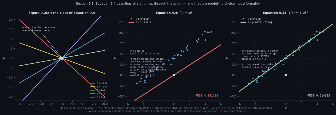
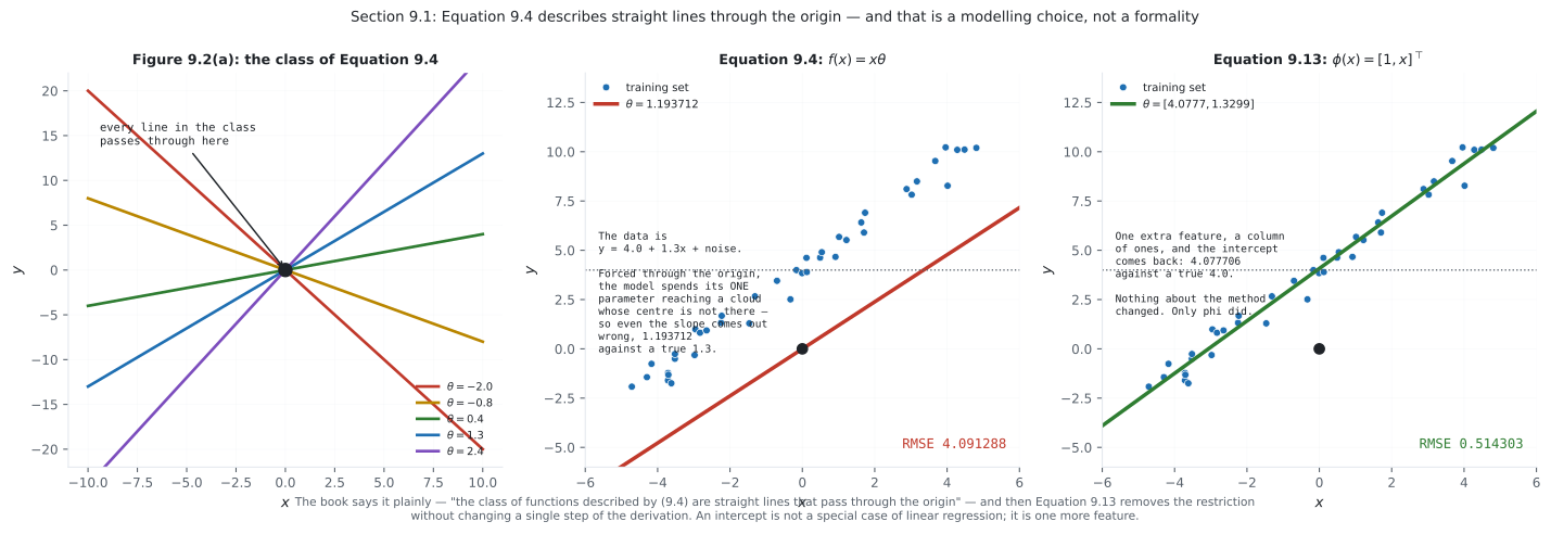
Reading the plot

The first figure takes a caption the book states once and prices it. The left panel is Figure 9.2(a) rebuilt — five members of Equation 9.4’s model class, and they all pass through a single point, because $f(0) = 0 \cdot \theta = 0$ for every $\theta$. The class is one-dimensional and pinned.

The middle and right panels are the cost. Given data that genuinely is $y = 4.0 + 1.3x + \epsilon$, Equation 9.4’s best fit reaches RMSE $4.091288$; adding one column of ones reaches $0.514303$ — close to the noise floor of $\sigma = 0.6$, which is as well as anything can do.

The detail worth carrying is not the intercept. It is that the slope also comes out wrong: $1.193712$ against a true $1.3$. The one-parameter model has a single knob and must use it both to set the tilt and to drag the line toward a cloud centred at $y \approx 4$. Those demands conflict, and the compromise corrupts the parameter that was in the model. A missing feature is not a localised error — it leaks into every coefficient you kept, which is page 805’s non-monotone slope arriving from a completely different direction.

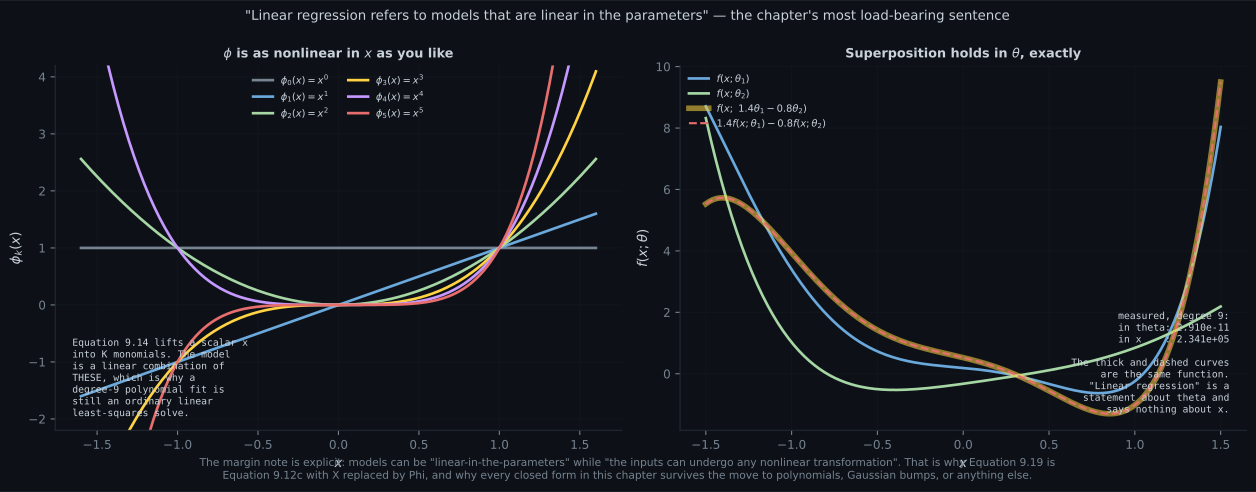
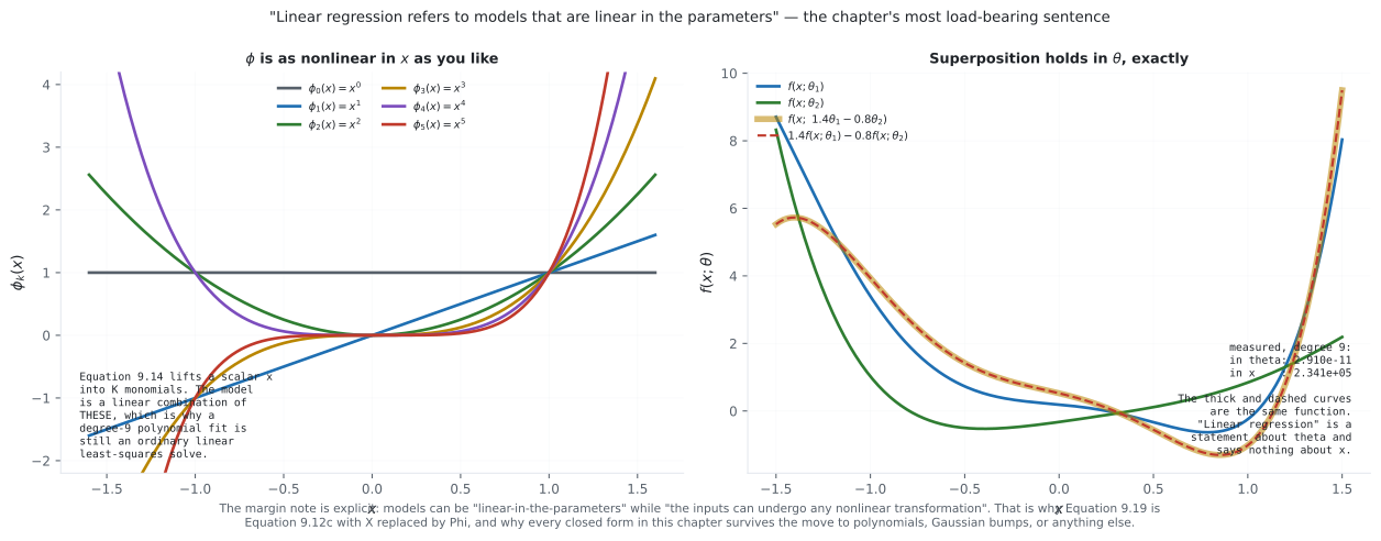
The second figure is the sentence the chapter repeats three times, turned into two numbers. Left: the monomial features $1, x, x^2, \ldots$ are as nonlinear in $x$ as anything you would want. Right: two random parameter vectors, their weighted combination drawn thick, and the same combination formed the other way drawn dashed on top. They coincide — measured, to $4.366\times10^{-11}$ at degree 9, while superposition in $x$ fails by $2.341\times10^{5}$.

That gap of sixteen orders of magnitude is the licence for everything that follows. $\boldsymbol\Phi$ can hold monomials, Gaussian bumps, wavelets, or the output of a fixed neural network, and the estimator stays $(\boldsymbol\Phi^\top\boldsymbol\Phi)^{-1}\boldsymbol\Phi^\top\mathbf{y}$. The word “linear” constrains how $\boldsymbol\theta$ enters, and nothing else.

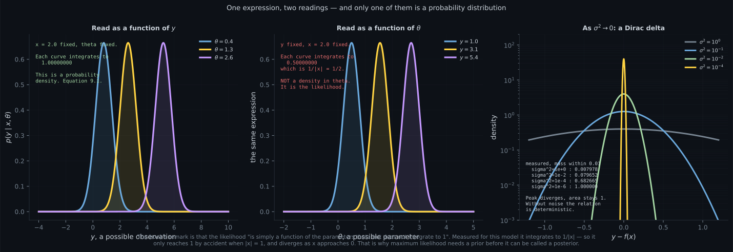
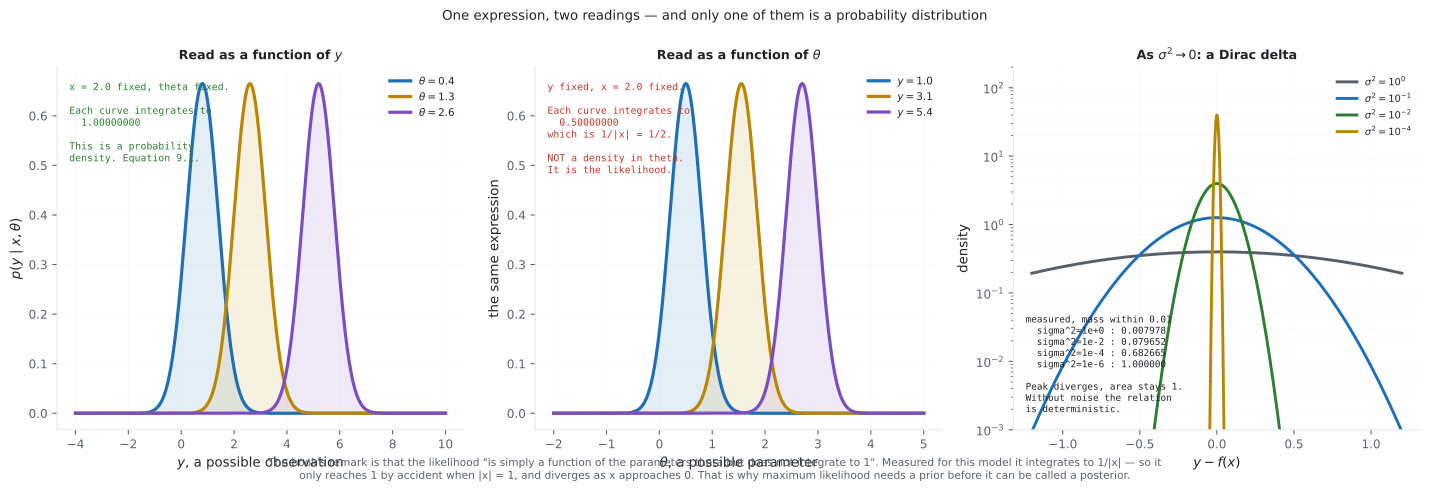
The third figure separates two objects that share a formula, and the middle panel has the sharper result than I expected. Over $y$, each curve integrates to $1.00000000$ — a probability density, as Equation 9.1 says. Over $\boldsymbol\theta$, the same expression integrates to $0.50000000$.

That is not “roughly less than one”. Substituting $u = x\theta$ gives $d\theta = du/\lvert x\rvert$, so the integral is exactly $1/\lvert x\rvert$ for every $x \neq 0$. Two consequences follow immediately. It equals $1$ only when $\lvert x\rvert = 1$ — a coincidence, not a property. And as $x \to 0$ it diverges, which is the book’s “may not even be integrable with respect to $\boldsymbol\theta$” with a specific failure mode attached.

Why this matters three sections from now: the missing normaliser is exactly what §9.3.3 has to supply to turn a likelihood into a posterior, and computing it is the entire content of §9.3.5. Maximum likelihood gets away with ignoring it because an argmax does not care about scale. Nothing else does.

The right panel is the Dirac limit, and the three columns say it precisely: the peak rises without bound ($0.3989 \to 398.9423$), the area never moves ($1.00000000$), and the mass within $\pm 0.01$ of the mean climbs from $0.007978$ to $1.000000$. A delta is not a tall Gaussian; it is the limit of a family whose area is conserved while its support collapses.

From the book

This page covers §9.1 and the opening of §9.2 of Mathematics for Machine Learning by Deisenroth, Faisal and Ong (draft of 2019-12-11). Equations 9.1–9.4 set up the likelihood, the noise model and the linear case, with the statement that Eq 9.4’s class is “straight lines that pass through the origin” and the margin note on the Dirac delta as “a Gaussian in the limit of $\sigma^2 \to 0$”. Example 9.1 and Figure 9.2 give the model class, the training set and the maximum likelihood fit. The margin notes that “linear regression refers to models that are linear in the parameters” and that “the inputs can undergo any nonlinear transformation” are the book’s, as is the definition of a feature as “a representation $\phi(x)$ of the inputs”. §9.2 gives the training set, Figure 9.3’s graphical model with shaded observed nodes, the conditional independence claim, the factorization 9.5, and the predictive 9.6. §9.2.1 supplies 9.7, the remark that the likelihood “is not a probability distribution in $\boldsymbol\theta$” and “may not even be integrable”, and the log-transform remark about numerical underflow and “very small numbers, such as $10^{-256}$”. The RMSE comparison of the two model classes, the exact value $1/\lvert x\rvert$ for the likelihood’s integral over $\boldsymbol\theta$, the superposition measurements, the underflow table and the Dirac-limit table are this module’s additions.

Compare

	as a function of $y$	as a function of $\boldsymbol\theta$
what it is called	the predictive distribution	the likelihood
integrates to	$1.00000000$	$1/\lvert x\rvert$, measured $0.50000000$
is it a density	yes	no
always integrable	yes	no — diverges as $x \to 0$
what you do with it	sample, form intervals	maximise (§9.2.1), multiply by a prior (§9.2.3)
the missing piece	—	the normaliser, supplied in §9.3.3 and computed in §9.3.5

	Eq 9.4, $f(x) = x^\top\boldsymbol\theta$	Eq 9.13, $f(x) = \phi^\top(x)\boldsymbol\theta$
model class	straight lines through the origin	anything spanned by $\phi$
linear in $\boldsymbol\theta$	yes	yes — unchanged
linear in $x$	yes	no, and it need not be
the estimator	$(\mathbf{X}^\top\mathbf{X})^{-1}\mathbf{X}^\top\mathbf{y}$, Eq 9.12c	$(\boldsymbol\Phi^\top\boldsymbol\Phi)^{-1}\boldsymbol\Phi^\top\mathbf{y}$, Eq 9.19
invertibility needs	$\mathrm{rk}(\mathbf{X}) = D$	$\mathrm{rk}(\boldsymbol\Phi) = K$
measured RMSE here	$4.091288$	$0.514303$

pch.quizTag Is the setup clear?

1. Equation 9.4 describes which class of functions?

   A All straight lines B Straight lines that pass through the origin — there is no intercept C All polynomials of degree at most D D All continuous functions
   pch.quizShowAnswer

   B — Straight lines that pass through the origin — there is no intercept — Measured on data that really is y = 4.0 + 1.3x: the one-parameter model reaches RMSE 4.091288 against 0.514303 for a model with a column of ones. And the damage is not confined to the intercept — the slope comes out at 1.193712 against a true 1.3, because one knob cannot serve two purposes.

2. What does 'linear regression' actually constrain?

   A That the model is a straight line in x B That the parameters enter linearly — the inputs may undergo any nonlinear transformation C That the noise is Gaussian D That there are at most two parameters
   pch.quizShowAnswer

   B — That the parameters enter linearly — the inputs may undergo any nonlinear transformation — Measured on a degree-9 model: superposition holds in theta to 4.366e-11 and fails in x by 2.341e+05. That is why Equation 9.19 is Equation 9.12c with X replaced by Phi and nothing else changed — Phi can hold monomials, Gaussian bumps, or the output of a fixed network.

3. The book says the likelihood is not a probability distribution in theta. Integrated over theta, what does it actually come to for this model?

   A Always 1, the book is being pedantic B Exactly 1 over the absolute value of x — measured at 0.50000000 for x = 2 C Always 0 D It depends on the noise variance
   pch.quizShowAnswer

   B — Exactly 1 over the absolute value of x — measured at 0.50000000 for x = 2 — Substituting u = x*theta gives d-theta = du over |x|. So it reaches 1 only by accident when |x| = 1, and diverges as x approaches zero — the book's 'may not even be integrable', with a specific failure mode. Maximum likelihood gets away with this because an argmax ignores scale; Section 9.3.3 does not.

4. Why does the chapter minimise the negative LOG-likelihood rather than maximise the likelihood directly?

   A Purely for mathematical elegance B Underflow: measured, the product of N densities is exactly 0.0 in float64 by N = 1000, and a gradient of zero is no gradient C Because the log-likelihood has a different minimiser D Because logs are faster to compute
   pch.quizShowAnswer

   B — Underflow: measured, the product of N densities is exactly 0.0 in float64 by N = 1000, and a gradient of zero is no gradient — The book gives both reasons: it 'does not suffer from numerical underflow' and 'the differentiation rules will turn out simpler', since the log turns a product into a sum whose gradient is a sum of individual gradients rather than a repeated product rule. The smallest positive float64 is 4.94e-324 and a thousand typical densities multiply straight past it.

5. Equation 9.6 gives the predictive distribution at a test input. How does its width vary with the test input?

   A It grows as you move away from the training data B It does not vary at all — it is sigma everywhere, measured at a 95 percent width of 2.351957 at x = 0 and at x = 100 C It shrinks with distance D It depends on the number of training points
   pch.quizShowAnswer

   B — It does not vary at all — it is sigma everywhere, measured at a 95 percent width of 2.351957 at x = 0 and at x = 100 — Equation 9.6 substitutes a point estimate into the likelihood, so the only uncertainty left is the observation noise. This is exactly the plug-in predictive Chapter 8 measured at 0.1796 coverage in far extrapolation while labelled 95 percent — and Section 9.3 is the chapter's answer to it.

6. Equation 9.5 factorizes the likelihood into a product over data points. What licenses that?

   A The Gaussian assumption alone B Conditional independence of y_i and y_j given their respective inputs — verified to 1.4e-15 C The fact that the inputs are sorted D It is an approximation that improves with N
   pch.quizShowAnswer

   B — Conditional independence of y_i and y_j given their respective inputs — verified to 1.4e-15 — That is what Figure 9.3's plate asserts, and page 807 measured the same equality for the Bernoulli case. Statistical independence means the distribution factorizes — the joint as one 12-dimensional Gaussian and as 12 separate factors agree to relative 1.399e-15.

Pitfalls

Assuming Equation 9.4 has an intercept

It does not. Measured: on data with a true intercept of $4.0$, the one-parameter model reaches RMSE $4.091288$ against $0.514303$, and its slope is wrong by $0.106288$ as well. Use Equation 9.13 with $\phi(x) = [1, x]^\top$ — an intercept is not a special case, it is one more feature.

Reading “linear regression” as “fits a straight line”

It means linear in the parameters. Measured: superposition holds in $\boldsymbol\theta$ to $4.4\times10^{-11}$ and fails in $x$ by $2.3\times10^{5}$ for the same degree-9 model. Polynomial regression, radial basis functions and a fixed feature extractor are all linear regression.

Treating the likelihood as a distribution over parameters

It integrates to $1/\lvert x\rvert$ — measured $0.50000000$ at $x = 2$ — and diverges as $x \to 0$. An argmax survives this; a posterior does not. The normaliser is what §9.3.3 supplies and §9.3.5 computes, and it is the single most expensive object in the chapter.

Multiplying densities instead of adding logs

Measured: the product of $N$ Gaussian densities is exactly $0.0$ in float64 by $N = 1000$, while the sum of logs is $-898.461655$. Underflow does not produce a small gradient; it produces none. The book’s second reason matters too — the log turns one product rule over $N$ terms into $N$ independent gradients.

Quoting Equation 9.6’s interval far from the data

Its width is $2 \times 1.96 \times \sigma$ at every test input — $2.351957$ at $x = 0$ and at $x = 100$ alike. Page 806 measured a plug-in interval of this kind at $0.1796$ coverage in far extrapolation while labelled $95\%$. §9.3.4’s Equation 9.68 is the fix, and the difference is one extra term.

Forgetting that sigma squared is assumed known

§9.1 says so explicitly, and the assumption is load-bearing: it is what lets §9.2.2 “ignore the scaling by $1/\sigma^2$”. Equation 9.22 estimates it, and the estimate is biased — page 902 measures by how much.

🧪 Try It Yourself

Exercise 1 – What the origin costs

pch.exerciseTag pch.exerciseTitle

Exercise 2 – The plate is a product

pch.exerciseTag pch.exerciseTitle

Exercise 3 – Why logs

pch.exerciseTag pch.exerciseTitle

Exercise 4 – It integrates to one over the magnitude of x

pch.exerciseTag pch.exerciseTitle

Exercise 5 – Linear in which argument?

pch.exerciseTag pch.exerciseTitle

Recall card

• Equation 9.1 models the noise explicitly rather than choosing a loss. Everything else in the chapter is a consequence of that one decision.
• Equation 9.2: y equals f of x plus i.i.d. zero-mean Gaussian noise of variance sigma squared. Sigma squared is assumed KNOWN for most of the chapter.
• Equation 9.4’s model class is straight lines through the origin. Measured on data with a true intercept of 4.0: RMSE 4.091288 against 0.514303, and the slope itself comes out at 1.193712 against a true 1.3.
• A missing feature is not a localised error. It leaks into the coefficients you kept, because the remaining parameters must compensate.
• Linear regression means linear in the PARAMETERS. Superposition in theta holds to 4.366e-11; in x it fails by 2.341e+05. A feature is any representation phi of the inputs, and it may be as nonlinear as you like.
• Equation 9.5: the likelihood factorizes because y_i and y_j are conditionally independent given their inputs. Verified to a relative 1.399e-15. That is what Figure 9.3’s plate asserts.
• The log-transform is not cosmetic. The product of N densities is exactly 0.0 in float64 by N = 1000; the sum of logs is an ordinary number at every N. The log also turns one product rule over N terms into N independent gradients.
• The likelihood is a density in y and not in theta. Over y it integrates to 1.00000000; over theta it integrates to exactly 1 over the absolute value of x — measured at 0.50000000 for x = 2, and it diverges as x approaches zero.
• The missing normaliser is the marginal likelihood. Maximum likelihood ignores it because an argmax ignores scale; Section 9.3.3 cannot, and Section 9.3.5 is the whole job of computing it.
• Equation 9.6’s predictive width is sigma everywhere — a 95 percent width of 2.351957 at x = 0 and at x = 100 alike. That is the plug-in interval Chapter 8 measured at 0.1796 coverage in extrapolation.
• Without noise, Equation 9.3 becomes a Dirac delta. Measured as sigma squared falls from 1 to 1e-6: the peak rises from 0.3989 to 398.9423, the area stays at 1.00000000, and the mass within plus or minus 0.01 climbs from 0.007978 to 1.000000.
• The negative log-likelihood is quadratic in theta, which is why a unique global solution exists and iterative gradient descent is unnecessary here.

Next: solve it. Maximum Likelihood Estimation for Linear Regression