Backpropagation and Optimizers (Adam, SGD)

Backpropagation is the chain rule applied in one particular order. Optimizers are what you do with the result. This page derives the first from scratch, checks it against TensorFlow to eight decimal places, then measures all seven Keras optimizers on the same problem — where the answer is not the one the folklore gives.

What you’ll learn

• Backpropagation derived layer by layer and matched to GradientTape within 7.45e-09.
• Why softmax and cross-entropy collapse into $\hat{p} - y$, so the output layer needs no chain rule at all.
• Momentum implemented by hand, matching Keras to 0.00e+00, and why it can take steps 10× the size of plain SGD.
• Adam implemented by hand to 1.97e-06, and what bias correction fixes: a first step 3.16× too large, growing to 6.5× by step 10.
• Seven optimizers measured: RMSprop 0.8565, Nadam 0.8525, Adam 0.8445, SGD 0.8425, AdaGrad 0.8265.
• The real difference: epochs to reach 0.84 ranged from 5 to never.
• What optimizer state costs — measured at 0, 1× and 2× the parameter count.

The training loop

diagram Diagram mermaid

  flowchart LR
  A["mini-batch"] --> B["forward pass
store every intermediate"]
  B --> C["loss
one number"]
  C --> D["backward pass
chain rule, output to input"]
  D --> E["gradients
one per parameter"]
  E --> F["optimizer
gradient -> update"]
  F --> G["new weights"]
  G --> A

The forward pass has to keep its intermediate activations, because the backward pass needs them. That is why training a model costs several times the memory of running one.

Backpropagation, one layer at a time

Take a two-layer classifier: $\mathbf{z}_1 = \mathbf{x}W_1 + \mathbf{b}_1$, $\mathbf{a}_1 = \text{relu}(\mathbf{z}_1)$, $\mathbf{z}_2 = \mathbf{a}_1 W_2 + \mathbf{b}_2$, then softmax and cross-entropy. Differentiating from the loss backwards:

$$\frac{\partial L}{\partial \mathbf{z}_2} = \frac{\hat{p} - y}{N} \qquad \frac{\partial L}{\partial W_2} = \mathbf{a}_1^{\top} \frac{\partial L}{\partial \mathbf{z}_2} \qquad \frac{\partial L}{\partial \mathbf{a}_1} = \frac{\partial L}{\partial \mathbf{z}_2} W_2^{\top}$$ $$\frac{\partial L}{\partial \mathbf{z}_1} = \frac{\partial L}{\partial \mathbf{a}_1} \odot \mathbb{1}[\mathbf{z}_1 > 0] \qquad \frac{\partial L}{\partial W_1} = \mathbf{x}^{\top} \frac{\partial L}{\partial \mathbf{z}_1}$$

The first expression is the one worth staring at. Softmax’s Jacobian is a full matrix and cross-entropy’s derivative is $-1/\hat{p}$; multiplied together they collapse to $\hat{p} - y$. The output layer’s gradient is just the prediction error, which is the same cancellation that makes sigmoid pair with binary cross-entropy on the loss functions page.

Implemented in twelve lines of NumPy and checked against TensorFlow on four rows:

Quantity	max |mine − TensorFlow|
loss	0.763195 vs 0.763195
$\partial L/\partial W_1$	7.45e−09
$\partial L/\partial \mathbf{b}_1$	7.45e−09
$\partial L/\partial W_2$	1.49e−08
$\partial L/\partial \mathbf{b}_2$	2.98e−08

Those residuals are float32 rounding, not disagreement. If you have worked through Autograd from Scratch, this is the same machinery specialised to a known architecture — hand-written backprop is what autodiff generates for you.

Two properties of this recipe matter later:

• Every layer’s gradient is a product of the layers above it. Twenty layers means a product of twenty terms, which is why depth causes vanishing and exploding gradients.
• Cost is one forward pass plus roughly two forward passes’ worth of backward work, independent of the parameter count — the property that makes training large models possible at all.

From gradient to update

SGD

$$\theta \leftarrow \theta - \eta \, \nabla_\theta L$$

No state, one hyperparameter, and the behaviour derived on the gradient descent page: stable while $\eta < 2/c$ for curvature $c$, and one rate has to satisfy the tightest direction.

Momentum

$$\mathbf{v} \leftarrow \beta \mathbf{v} - \eta \nabla_\theta L \qquad \theta \leftarrow \theta + \mathbf{v}$$

Implemented by hand and compared to SGD(0.05, momentum=0.9) step by step on $L(a,b) = a^2 + 10b^2$:

Step	my $a$	my $b$	Keras $a$	Keras $b$
1	2.340000	0.000000	2.340000	0.000000
2	1.872000	−0.900000	1.872000	−0.900000
3	1.263600	−0.810000	1.263600	−0.810000
5	−0.075816	0.801900	−0.075816	0.801900

Difference: 0.00e+00. Look at the $b$ column: it goes 0.000, −0.900, −0.810, then back positive. Momentum has overshot the minimum and is oscillating. With a constant gradient the velocity converges to $\eta g / (1 - \beta)$, so at $\beta = 0.9$ steps grow up to 10× plain SGD’s. That is the whole point — and the whole risk.

Nesterov

Evaluate the gradient at $\theta + \beta\mathbf{v}$ instead of $\theta$: measure the slope where the momentum is about to put you, not where you already are. It is a one-line change and usually converges slightly faster.

AdaGrad

$$\mathbf{s} \leftarrow \mathbf{s} + (\nabla_\theta L)^2 \qquad \theta \leftarrow \theta - \frac{\eta}{\sqrt{\mathbf{s}} + \epsilon} \nabla_\theta L$$

Per-parameter rates: directions with big gradients get scaled down. The flaw is structural — $\mathbf{s}$ only ever grows, so the effective learning rate decays monotonically toward zero and the run can stop before it arrives. The measurement below shows exactly that.

RMSprop

$$\mathbf{s} \leftarrow \rho \mathbf{s} + (1 - \rho)(\nabla_\theta L)^2$$

The same idea with a decaying average instead of a running sum, so the effective rate can recover. One character of maths, and it is the difference between finishing and stalling.

Adam

Momentum and RMSprop together, each with bias correction:

$$\mathbf{m} \leftarrow \beta_1 \mathbf{m} + (1-\beta_1)\nabla_\theta L \qquad \mathbf{s} \leftarrow \beta_2 \mathbf{s} + (1-\beta_2)(\nabla_\theta L)^2$$ $$\hat{\mathbf{m}} = \frac{\mathbf{m}}{1 - \beta_1^t} \qquad \hat{\mathbf{s}} = \frac{\mathbf{s}}{1 - \beta_2^t} \qquad \theta \leftarrow \theta - \eta \frac{\hat{\mathbf{m}}}{\sqrt{\hat{\mathbf{s}}} + \epsilon}$$

Hand-implemented, it matches keras.optimizers.Adam to 1.97e-06 over five steps — float32 against float64, not a disagreement.

What bias correction is for. Both $\mathbf{m}$ and $\mathbf{s}$ start at zero, so early estimates are biased low — but by different factors, because $\beta_1 = 0.9$ and $\beta_2 = 0.999$. With a constant gradient of 1.0 and $\eta = 0.05$:

Step	Uncorrected step size	Corrected step size
1	0.158113 (3.16× η)	0.050000
2	0.212479 (4.25× η)	0.050000
5	0.289857 (5.80× η)	0.050000
10	0.326394 (6.53× η)	0.050000

Without the correction the first update is over three times the requested learning rate, and it keeps growing for dozens of steps. With it, a constant gradient gives exactly the learning rate. Bias correction is not a refinement; it is what makes $\eta$ mean what it says during the early steps when the model is most fragile.

Nadam

Adam with the Nesterov look-ahead. Same state, same cost.

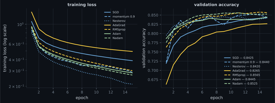
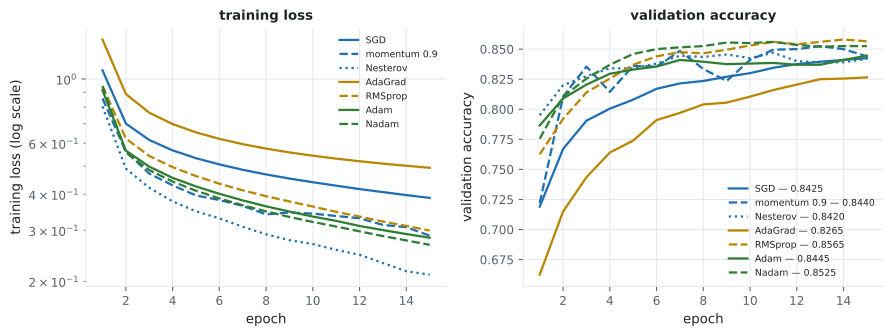
What they actually do on a real problem

Fashion-MNIST, 8,000 rows, one hidden layer of 128 ReLU units (101,770 parameters), batch 128, 15 epochs, one seed, everything else identical.

figure Seven optimizers, one architecture, one seed matplotlib

Blue is the SGD family, amber the accumulating methods, green the Adam family. In the accuracy panel every optimizer except AdaGrad finishes inside a 0.014 band — but they arrive at very different times. Nesterov reaches the lowest training loss (0.2108) while finishing joint-lowest on validation accuracy, which is overfitting, not superiority.

Optimizer	Final training loss	Final val accuracy	Best val accuracy	Epochs to 0.84	Seconds
SGD	0.388167	0.8425	0.8425	14	5.91
momentum 0.9	0.287497	0.8440	0.8525	7	5.94
Nesterov	0.210798	0.8420	0.8470	7	6.19
AdaGrad	0.493285	0.8265	0.8265	never	6.30
RMSprop	0.299386	0.8565	0.8580	6	6.21
Adam	0.282805	0.8445	0.8445	7	6.59
Nadam	0.267235	0.8525	0.8560	5	6.81

Four honest readings:

1. Adam did not win. RMSprop finished 0.0120 ahead of it and Nadam 0.0080 ahead. Adam beat plain SGD by 0.0020 — a difference no one should act on from a single run.
2. The real gap is speed, not accuracy. Nadam reached 0.84 in 5 epochs; plain SGD needed 14. If your budget is 5 epochs, that gap is the entire result. If it is 15, most of it has evaporated.
3. AdaGrad never arrived. Its accumulating denominator drove the effective rate toward zero, and it finished 0.0300 behind everything else. This is the textbook failure, reproduced exactly.
4. The lowest training loss lost. Nesterov’s 0.2108 was the best training loss and its validation accuracy was joint-lowest. Training loss ranks how well an optimiser descends, which is not the question you are asking.

Why the adaptive methods move differently

figure The same bowl, four update rules, 60 steps each matplotlib

L(a,b) = a² + 10b², so the b direction is ten times steeper. SGD kills b immediately and then crawls along a, reaching 2.18e-05. Momentum overshoots b repeatedly and ends at 1.91e-02. RMSprop and Adam scale each axis by its own gradient history and take almost straight paths — yet finish at 1.25e-02 and 9.71e-02, worse than plain SGD on this clean quadratic.

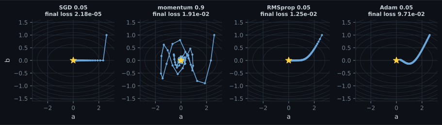
Update rule	Final loss after 60 steps
SGD 0.05	2.1830e−05
momentum 0.9	1.9110e−02
RMSprop 0.05	1.2478e−02
Adam 0.05	9.7094e−02

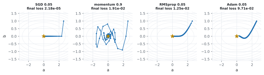
On a perfectly conditioned two-parameter quadratic with a well-chosen rate, plain SGD wins by three orders of magnitude. Adaptive methods pay for their robustness with a floor on how precisely they converge — the $\epsilon$ in the denominator and the momentum term both keep them moving near the optimum. Their advantage appears when curvature varies wildly between parameters and you cannot tune a rate per axis by hand, which is every real network and no toy quadratic.

sketch Momentum, one slider p5.js Pause Restart

Gradient descent on the same anisotropic bowl. Drag the beta slider from 0 (plain SGD) upward and watch the path change from a slow crawl to an overshooting zig-zag.

What the optimizer costs in memory

Measured on the 101,770-parameter model by counting the optimizer’s own variables after one step:

Optimizer	Slot values stored	Ratio to parameters
SGD	0	0.00
momentum	101,770	1.00
RMSprop	101,770	1.00
Adam	203,540	2.00

figure What the optimizer costs before a single activation is stored matplotlib

A 100M-parameter model is 0.40 GB of float32 weights. Momentum, AdaGrad and RMSprop double that to 0.80 GB; Adam and Nadam triple it to 1.20 GB. Add gradients and stored activations and this is why the batch size you can fit depends on which optimizer you chose.

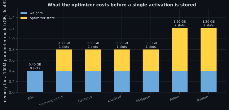
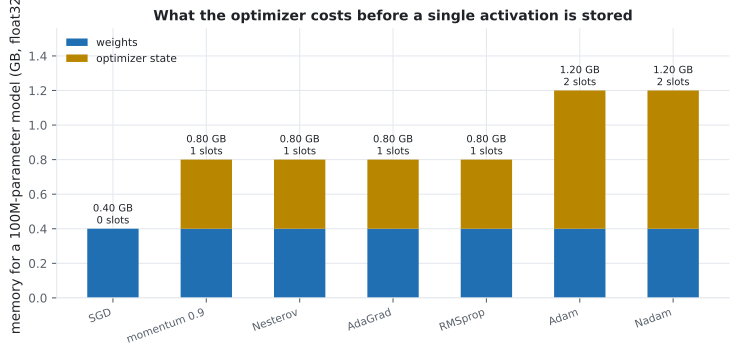
Wall-clock time barely noticed the difference — 5.91s for SGD against 6.81s for Nadam, a 15% spread, on a model this small. Memory is the constraint that actually bites: choosing Adam over SGD costs 0.80 GB on a 100M-parameter model before a single activation is stored.

Choosing one

• Start with Adam at its defaults (1e-3, $\beta_1=0.9$, $\beta_2=0.999$). It is the most forgiving of a badly chosen learning rate, which is the failure mode you are most likely to hit.
• Try RMSprop and Nadam if you have budget for a second run. Here they were the best two, and they cost nothing to test.
• Reach for SGD with momentum when you can afford to tune the rate and a schedule. Well-tuned SGD is still the state of the art for large vision models, and it is the cheapest in memory.
• Skip AdaGrad for deep networks. Its accumulating denominator is the failure reproduced above.
• Do not act on 0.002 accuracy differences. Above, SGD-versus-Adam is 0.0020 from one seed. Run several seeds before believing any ranking.

sketch The measured table, ranked p5.js Pause Restart

Click a column to rank every row by it. The bars are that column's values and the highest and lowest are computed from the numbers, not written in.

Pitfalls

• Assuming Adam is always best. RMSprop beat it by 0.0120 and Nadam by 0.0080 in the run above.
• Comparing optimizers by training loss. Nesterov had the lowest training loss and the joint-lowest validation accuracy.
• Using AdaGrad on a deep network. The effective rate decays monotonically; it never reached 0.84 here.
• Reusing SGD’s learning rate for Adam or vice versa. SGD wanted 0.1 in these runs; Adam wanted 0.001 — a factor of 100.
• Forgetting momentum’s step multiplier. At $\beta = 0.9$, steps reach 10× plain SGD’s. A rate that was stable without momentum can diverge with it.
• Implementing Adam without bias correction. The first step comes out 3.16× too large and stays inflated for dozens of steps.
• Budgeting memory for weights only. Adam needs 3× the weight memory, before gradients and activations.
• Reusing an optimizer object across models. Its slots are shaped to the parameters it first saw. Build a fresh one per model.

Recap

• Backpropagation is the chain rule evaluated output-to-input; softmax with cross-entropy collapses to $\hat{p} - y$, verified against TensorFlow to 7.45e-09.
• Momentum accumulates a velocity, taking steps up to $1/(1-\beta)$ times plain SGD’s, and can overshoot.
• AdaGrad’s denominator only grows, so its effective rate decays to zero; RMSprop replaces the sum with a decaying average and fixes it.
• Adam is momentum plus RMSprop plus bias correction; without the correction the first step is 3.16× the requested rate.
• Measured on Fashion-MNIST: RMSprop 0.8565, Nadam 0.8525, Adam 0.8445, SGD 0.8425, AdaGrad 0.8265 — a 0.014 band excluding AdaGrad.
• Epochs to reach 0.84 ranged from 5 (Nadam) to 14 (SGD) to never (AdaGrad). That is the difference worth caring about.
• On a clean quadratic, plain SGD beat all three adaptive methods by orders of magnitude. Adaptivity buys robustness, not precision.
• Optimizer state costs 0, 1× or 2× the parameter count: 0.40, 0.80 or 1.20 GB for a 100M-parameter model.

Next

Every gradient above was a product of the layers above it. Stack twenty layers and that product either collapses or explodes: Vanishing & Exploding Gradients.

pch.quizTag pch.quizDefaultTitle

1. Why does the output layer's gradient for softmax + cross-entropy reduce to (p - y), with no chain-rule product?

   A Because softmax has no derivative B Because softmax's Jacobian and cross-entropy's -1/p derivative cancel exactly when multiplied, leaving the plain prediction error C Because Keras special-cases that combination internally D Because the loss is averaged over the batch
   pch.quizShowAnswer

   B — Because softmax's Jacobian and cross-entropy's -1/p derivative cancel exactly when multiplied, leaving the plain prediction error — The same cancellation makes sigmoid pair with binary cross-entropy. It is why these pairings are standard rather than arbitrary.

2. AdaGrad never reached 0.84 validation accuracy in 15 epochs while every other optimizer did. What is the mechanism?

   A Its learning rate was set too low at 0.01 B AdaGrad accumulates the sum of squared gradients, and since that sum only grows, the effective learning rate decays monotonically toward zero and training stalls C AdaGrad cannot handle ReLU activations D It needs a larger batch size to work
   pch.quizShowAnswer

   B — AdaGrad accumulates the sum of squared gradients, and since that sum only grows, the effective learning rate decays monotonically toward zero and training stalls — RMSprop replaces the running sum with a decaying average, which lets the effective rate recover. That single change is the fix.

3. Nadam reached 0.84 accuracy in 5 epochs and plain SGD needed 14, yet their final accuracies were 0.8525 and 0.8425. What should you conclude?

   A Nadam is strictly better and SGD should not be used B Adaptive methods mainly buy time-to-target rather than final accuracy — which matters enormously on a 5-epoch budget and much less on a 15-epoch one C The SGD run was misconfigured D Final accuracy is the only number that matters
   pch.quizShowAnswer

   B — Adaptive methods mainly buy time-to-target rather than final accuracy — which matters enormously on a 5-epoch budget and much less on a 15-epoch one — Both readings are in the same table. Which one is decisive depends entirely on your compute budget.

4. Adam without bias correction takes a first step 3.16x larger than the learning rate. Why?

   A Because the gradient is largest at the start of training B Because m and s both start at zero and are therefore biased low, but by different factors since beta_1 = 0.9 and beta_2 = 0.999 — the ratio m/sqrt(s) is inflated until both have warmed up C Because epsilon is too small in the denominator D Because the learning rate is applied twice on the first step
   pch.quizShowAnswer

   B — Because m and s both start at zero and are therefore biased low, but by different factors since beta_1 = 0.9 and beta_2 = 0.999 — the ratio m/sqrt(s) is inflated until both have warmed up — Dividing each by (1 - beta^t) removes the bias, so a constant gradient produces a step of exactly the learning rate from step one.

5. You are fine-tuning a 100M-parameter model and running out of memory. What does switching from Adam to SGD with momentum save?

   A Nothing — optimizer choice does not affect memory B 0.40 GB: Adam stores two float32 slots per parameter (0.80 GB) against momentum's one (0.40 GB), on top of the 0.40 GB of weights C It halves the activation memory D It reduces the gradient memory to zero
   pch.quizShowAnswer

   B — 0.40 GB: Adam stores two float32 slots per parameter (0.80 GB) against momentum's one (0.40 GB), on top of the 0.40 GB of weights — Measured on the small model: SGD 0 slots, momentum and RMSprop 1x the parameter count, Adam 2x. That scales linearly.

🧪 Try It Yourself

pch.exerciseTag pch.exerciseTitle

pch.exerciseTag pch.exerciseTitle

pch.exerciseTag pch.exerciseTitle

pch.exerciseTag pch.exerciseTitle

pch.exerciseTag pch.exerciseTitle

pch.exerciseTag pch.exerciseTitle