Orthonormal Basis

A basis gives you coordinates. Chapter 2 showed how: to express $\mathbf{x}$ in a basis $\mathbf{B}$, solve $\mathbf{B}\boldsymbol{\lambda} = \mathbf{x}$. That solve is the price of a general basis, and it is a real price — it costs $O(n^3)$, it needs the basis to be well conditioned, and it has to be redone from scratch every time you add a basis vector.

An orthonormal basis removes the solve entirely. Coordinates become inner products, one per basis vector, computed independently. That is the whole point of this page, and it is why every serious numerical routine in the rest of the book — QR, eigendecomposition, SVD, PCA — hands you an orthonormal basis rather than any other kind.

What you’ll learn

• Definition 3.9, and the two conditions in it: pairwise orthogonal and unit length.
• Why $\mathbf{B}^\top\mathbf{B} = \mathbf{I}$ is the compact form of both conditions at once.
• Coordinates as inner products, and Parseval’s identity — the squared coordinates add up to the squared length.
• The Gram-Schmidt construction, and the book’s alternative route through Gaussian elimination on $[\tilde{\mathbf{B}}\tilde{\mathbf{B}}^\top \mid \tilde{\mathbf{B}}]$.
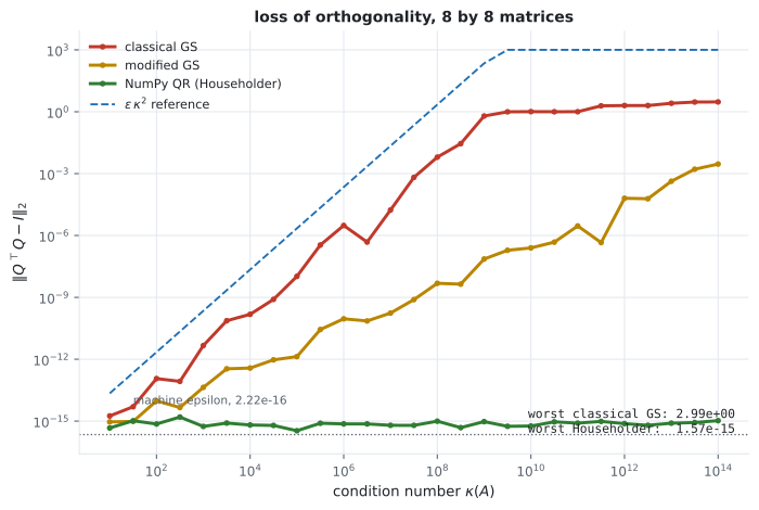
• The measured reason nobody implements textbook Gram-Schmidt: at condition number $10^{10}$ it loses orthogonality completely, while Householder QR does not budge from machine precision.

Intuition: a coordinate system where the axes do not lean on each other

Think about reading coordinates off a graph. If the axes are perpendicular and marked in equal units, reading a point’s $x$-coordinate is a single glance: drop a line straight down. Neither axis tells you anything about the other, so the two readings are independent.

Now skew the axes so they meet at $30°$. Dropping a line “straight down” no longer gives the $x$-coordinate, because moving along the second axis also changes your first coordinate. You have to solve for both at once, and the closer the axes get to parallel the more the two readings interfere — which is exactly what an ill-conditioned basis is.

An orthonormal basis is the first picture, in $n$ dimensions.

diagram Diagram mermaid

  flowchart TD
  B["a basis (b1, …, bn)"]
  B --> GEN["general basis:
coordinates need a SOLVE
Bλ = x, O(n³)"]
  B --> ORTH["pairwise orthogonal:
⟨bi, bj⟩ = 0 for i ≠ j"]
  ORTH --> UNIT["plus unit length:
⟨bi, bi⟩ = 1"]
  UNIT --> ONB["ORTHONORMAL BASIS
Def 3.9"]
  ONB --> GRAM["BᵀB = I
both conditions in one equation"]
  GRAM --> COORD["coordinates are inner products:
λ = Bᵀx, O(n²), no solve"]
  GRAM --> PARS["Parseval: Σ λi² = ‖x‖²"]
  GRAM --> INV["B⁻¹ = Bᵀ, so nothing is ever inverted"]
  COORD --> PROJ["projection collapses to BBᵀx
§3.8"]

The rightmost consequence is the one §3.8 will cash in: the general projection formula $\mathbf{B}(\mathbf{B}^\top\mathbf{B})^{-1}\mathbf{B}^\top$ collapses to $\mathbf{B}\mathbf{B}^\top$ when the basis is orthonormal, because the middle factor becomes the identity.

The math

Definition 3.9 — Orthonormal basis

Consider an $n$-dimensional vector space $V$ and a basis $\{\mathbf{b}_1, \dots, \mathbf{b}_n\}$ of $V$. If

$$\langle \mathbf{b}_i, \mathbf{b}_j \rangle = 0 \quad \text{for } i \neq j \tag{3.33}$$$$\langle \mathbf{b}_i, \mathbf{b}_i \rangle = 1 \tag{3.34}$$

for all $i, j$, then the basis is called an orthonormal basis (ONB). If only Equation 3.33 is satisfied, the basis is called an orthogonal basis.

Equation 3.34 says every basis vector has unit length, since $\lVert\mathbf{b}_i\rVert = \sqrt{\langle\mathbf{b}_i,\mathbf{b}_i\rangle} = 1$.

One equation instead of two

Stack the basis vectors as the columns of $\mathbf{B}$. Then the $(i,j)$ entry of $\mathbf{B}^\top\mathbf{B}$ is exactly $\langle\mathbf{b}_i, \mathbf{b}_j\rangle$, so Equations 3.33 and 3.34 together say

$$\mathbf{B}^\top\mathbf{B} = \mathbf{I} .$$

That matrix $\mathbf{B}^\top\mathbf{B}$ is called the Gram matrix of the basis, and “the basis is orthonormal” and “its Gram matrix is the identity” are the same statement. For a square $\mathbf{B}$ this also makes it an orthogonal matrix in the sense of Definition 3.8, so $\mathbf{B}^{-1} = \mathbf{B}^\top$.

Coordinates become inner products

For a general basis, the coordinates $\boldsymbol{\lambda}$ of $\mathbf{x}$ satisfy $\mathbf{B}\boldsymbol{\lambda} = \mathbf{x}$, so $\boldsymbol{\lambda} = (\mathbf{B}^\top\mathbf{B})^{-1}\mathbf{B}^\top\mathbf{x}$. When the basis is orthonormal the middle factor is $\mathbf{I}^{-1} = \mathbf{I}$ and this collapses to

$$\boldsymbol{\lambda} = \mathbf{B}^\top\mathbf{x}, \qquad\text{that is,}\qquad \lambda_i = \langle \mathbf{b}_i, \mathbf{x}\rangle .$$

Read the second form carefully. Each coordinate is computed from its own basis vector alone. No solve, no interference between coordinates, and — the part that matters for truncation — adding an $(n{+}1)$-th orthonormal direction does not change any of the first $n$ coordinates. That is why Fourier series, wavelets and PCA all truncate gracefully and a general basis expansion does not.

Parseval’s identity

$$\lVert \mathbf{x} \rVert^2 = \sum_{i=1}^{n} \lambda_i^2 \qquad\text{when } \mathbf{B} \text{ is orthonormal}$$

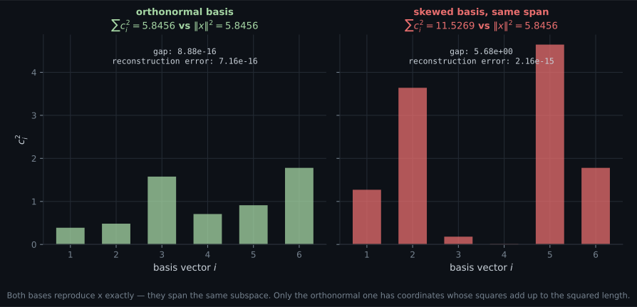
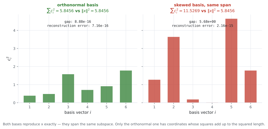
Expand $\lVert\mathbf{x}\rVert^2 = \lVert\mathbf{B}\boldsymbol{\lambda}\rVert^2 = \boldsymbol{\lambda}^\top\mathbf{B}^\top\mathbf{B}\boldsymbol{\lambda} = \boldsymbol{\lambda}^\top\boldsymbol{\lambda}$ and there it is. Under a non-orthonormal basis the middle factor is not the identity and the identity simply fails — measured below, the gap is $5.68$ on a vector of squared length $5.85$, which is a $97\%$ error rather than a rounding difference.

Gram-Schmidt

Equations 3.67 and 3.68 — Gram-Schmidt orthogonalisation

Given any basis $(\mathbf{b}_1, \dots, \mathbf{b}_n)$ of an $n$-dimensional vector space $V$, construct an orthogonal basis $(\mathbf{u}_1, \dots, \mathbf{u}_n)$ by

$$\mathbf{u}_1 := \mathbf{b}_1$$$$\mathbf{u}_k := \mathbf{b}_k - \pi_{\mathrm{span}[\mathbf{u}_1,\dots,\mathbf{u}_{k-1}]}(\mathbf{b}_k), \qquad k = 2, \dots, n$$

Normalising each $\mathbf{u}_k$ then gives an ONB. Such a basis always exists, and $\mathrm{span}[\mathbf{b}_1,\dots,\mathbf{b}_n] = \mathrm{span}[\mathbf{u}_1,\dots,\mathbf{u}_n]$ — the subspace is unchanged, only the axes are re-aimed.

The construction is one projection per step, so it belongs to §3.8; the book states it there and this page uses it. Two properties worth naming:

• The result depends on the order. $\mathbf{u}_1$ is $\mathbf{b}_1$ untouched, so whichever vector you list first survives unchanged. Different orders give different orthonormal bases of the same subspace.
• The span never changes. Every $\mathbf{u}_k$ is $\mathbf{b}_k$ minus a combination of earlier vectors, so nothing leaves the subspace and nothing new enters it.

The book’s other route

The book also mentions obtaining an ONB by applying Gaussian elimination to the augmented matrix $[\tilde{\mathbf{B}}\tilde{\mathbf{B}}^\top \mid \tilde{\mathbf{B}}]$, where $\tilde{\mathbf{B}}$ has the spanning vectors as columns. It is the same computation with the projections done all at once rather than one at a time, and it inherits the same numerical weakness — forming $\tilde{\mathbf{B}}\tilde{\mathbf{B}}^\top$ squares the condition number before any elimination happens.

From the book

Section 3.5 with Definition 3.9 (Equations 3.33 and 3.34) and Example 3.8 (Equation 3.35), which gives the orthonormal basis $\mathbf{b}_1 = \tfrac{1}{\sqrt{2}}(1,1)^\top$, $\mathbf{b}_2 = \tfrac{1}{\sqrt{2}}(1,-1)^\top$ of $\mathbb{R}^2$. The section also notes the $[\tilde{\mathbf{B}}\tilde{\mathbf{B}}^\top \mid \tilde{\mathbf{B}}]$ route. Gram-Schmidt itself is Section 3.8.3, Equations 3.67 and 3.68, with Example 3.12 and Figure 3.12. Chapter 4 mentions that the $\mathbf{U}$ and $\mathbf{V}$ of an SVD are orthonormal bases, and Chapter 10 relies on that.

Worked example by hand

Example 3.8 from the book

$$\mathbf{b}_1 = \frac{1}{\sqrt{2}}\begin{bmatrix}1\\1\end{bmatrix}, \qquad \mathbf{b}_2 = \frac{1}{\sqrt{2}}\begin{bmatrix}1\\-1\end{bmatrix}$$

check	working	result
$\langle\mathbf{b}_1,\mathbf{b}_2\rangle$	$\tfrac{1}{2}(1\cdot1 + 1\cdot(-1)) = \tfrac{1}{2}(1-1)$	$0$ — orthogonal
$\langle\mathbf{b}_1,\mathbf{b}_1\rangle$	$\tfrac{1}{2}(1+1)$	$1$ — unit length
$\langle\mathbf{b}_2,\mathbf{b}_2\rangle$	$\tfrac{1}{2}(1+1)$	$1$ — unit length

So $\mathbf{B}^\top\mathbf{B} = \mathbf{I}$ and this is an ONB. Now use it: take $\mathbf{x} = (3,-1)^\top$.

$$\lambda_1 = \langle\mathbf{b}_1,\mathbf{x}\rangle = \tfrac{1}{\sqrt{2}}(3 - 1) = \tfrac{2}{\sqrt{2}} = \sqrt{2} \approx 1.414214$$ $$\lambda_2 = \langle\mathbf{b}_2,\mathbf{x}\rangle = \tfrac{1}{\sqrt{2}}(3 + 1) = \tfrac{4}{\sqrt{2}} = 2\sqrt{2} \approx 2.828427$$

Two independent inner products, no system solved. Reconstruct to check: $\lambda_1\mathbf{b}_1 + \lambda_2\mathbf{b}_2 = \tfrac{\sqrt{2}}{\sqrt{2}}(1,1) + \tfrac{2\sqrt{2}}{\sqrt{2}}(1,-1) = (1,1) + (2,-2) = (3,-1)$. ✓

And Parseval: $\lVert\mathbf{x}\rVert^2 = 9 + 1 = 10$, while $\lambda_1^2 + \lambda_2^2 = 2 + 8 = 10$. ✓

The book’s Exercise 3.8, worked by Gram-Schmidt

Turn $\mathbf{b}_1 = (1,1,1)^\top$, $\mathbf{b}_2 = (-1,2,0)^\top$ into an ONB of the plane they span.

Step 1. $\mathbf{u}_1 := \mathbf{b}_1 = (1,1,1)^\top$.

Step 2. Subtract the projection of $\mathbf{b}_2$ onto $\mathbf{u}_1$:

$$\frac{\langle\mathbf{u}_1,\mathbf{b}_2\rangle}{\langle\mathbf{u}_1,\mathbf{u}_1\rangle} = \frac{-1 + 2 + 0}{1+1+1} = \frac{1}{3}$$ $$\mathbf{u}_2 = \mathbf{b}_2 - \tfrac{1}{3}\mathbf{u}_1 = \begin{bmatrix}-1\\2\\0\end{bmatrix} - \tfrac{1}{3}\begin{bmatrix}1\\1\\1\end{bmatrix} = \begin{bmatrix}-4/3\\5/3\\-1/3\end{bmatrix}$$

Confirm orthogonality: $\langle\mathbf{u}_1,\mathbf{u}_2\rangle = -\tfrac{4}{3} + \tfrac{5}{3} - \tfrac{1}{3} = 0$. ✓

Step 3. Normalise. $\lVert\mathbf{u}_1\rVert = \sqrt{3}$ and $\lVert\mathbf{u}_2\rVert = \tfrac{1}{3}\sqrt{16+25+1} = \tfrac{\sqrt{42}}{3} \approx 2.160247$, so

$$\mathbf{c}_1 = \frac{1}{\sqrt{3}}\begin{bmatrix}1\\1\\1\end{bmatrix}, \qquad \mathbf{c}_2 = \frac{1}{\sqrt{42}}\begin{bmatrix}-4\\5\\-1\end{bmatrix}$$

The $\tfrac{1}{3}$ cancels: $\tfrac{1}{\sqrt{42}/3}\cdot\tfrac{1}{3}(-4,5,-1) = \tfrac{1}{\sqrt{42}}(-4,5,-1)$.

onb_worked.py

import numpy as np
 
# Example 3.8
b1 = np.array([1.0, 1.0]) / np.sqrt(2)
b2 = np.array([1.0, -1.0]) / np.sqrt(2)
B = np.stack([b1, b2], axis=1)
print("B^T B =\n", np.round(B.T @ B, 15))
 
x = np.array([3.0, -1.0])
lam = B.T @ x                       # coordinates: two inner products, no solve
print("coordinates:", np.round(lam, 6))
print("reconstruct:", np.round(B @ lam, 6))
print("Parseval: |x|^2 =", float(x @ x), " sum lam^2 =", float((lam ** 2).sum()))
 
# Exercise 3.8: Gram-Schmidt
p1 = np.array([1.0, 1.0, 1.0])
p2 = np.array([-1.0, 2.0, 0.0])
u1 = p1.copy()
coeff = float(u1 @ p2) / float(u1 @ u1)
u2 = p2 - coeff * u1
print("coefficient:", coeff, " u2 =", u2, " <u1,u2> =", float(u1 @ u2))
c1, c2 = u1 / np.linalg.norm(u1), u2 / np.linalg.norm(u2)
print("||u2|| =", np.linalg.norm(u2), " sqrt(42)/3 =", np.sqrt(42) / 3)
print("c2 * sqrt(42) =", np.round(c2 * np.sqrt(42), 6))
C = np.stack([c1, c2], axis=1)
print("C^T C =\n", np.round(C.T @ C, 15))

output

B^T B =
 [[ 1. -0.]
 [-0.  1.]]
coordinates: [1.414214 2.828427]
reconstruct: [ 3. -1.]
Parseval: |x|^2 = 10.0  sum lam^2 = 9.999999999999998
coefficient: 0.3333333333333333  u2 = [-1.33333333  1.66666667 -0.33333333]  <u1,u2> = 1.6653345369377348e-16
||u2|| = 2.1602468994692865  sqrt(42)/3 = 2.160246899469287
c2 * sqrt(42) = [-4.  5. -1.]
C^T C =
 [[1. 0.]
 [0. 1.]]

Note the two residues of floating point. Parseval gives $9.999999999999998$ rather than $10$, and $\langle\mathbf{u}_1,\mathbf{u}_2\rangle$ is $1.67\times10^{-16}$ rather than $0$. Both are one or two units in the last place — the correct amount of disagreement for a computation involving a square root, not an error to chase.

See it move

The first sketch is the skewed-axes intuition, made numeric. Drag the second basis vector towards the first and watch the coordinate readings interfere; drag it perpendicular and they stop.

sketch Reading coordinates off leaning axes p5.js Pause Restart

Drag b2. The white point x is fixed. The amber and blue segments are its coordinates in the basis (b1, b2), obtained by solving. When b2 is perpendicular to b1 the coordinates equal the plain inner products, shown alongside; as b2 leans towards b1 the two diverge and the condition number climbs.

The second sketch is Gram-Schmidt with a draggable input. The grey shadow is the part being subtracted.

sketch Gram-Schmidt: subtract the shadow, keep the rest p5.js Pause Restart

u1 is fixed as b1. Drag b2 anywhere. The grey arrow is the projection of b2 onto u1 — the part of b2 that already points along u1 — and u2 is what is left after removing it. The readout confirms the inner product of u1 with u2 is zero for every position of b2, and the normalised pair is drawn on the unit circle.

And the stepped version, on the book’s own Exercise 3.8:

vectorExercise 3.8, step by stepGram-Schmidt, §3.8.3

dim U 0ambient R^3

1u = [b[0]]2for k in range(1, n):3    r = b[k]4    for uj in u:5        r = r - (uj @ b[k]) / (uj @ uj) * uj   # subtract the shadow6    u.append(r)                                # what is left is orthogonal7Q = [uj / norm(uj) for uj in u]                # normalise for an ONB

setup2 vectors that span the subspace but are not orthogonal to each other. Gram-Schmidt keeps the first one and repairs each of the others in turn, by subtracting off whatever part of it already points along the ones already accepted.

Play‹›1/5⟲

Two vectors spanning a plane in three dimensions, turned into an orthonormal pair. The final frame shows the Gram matrix, which is the identity.

From scratch

Two implementations that differ by one word, and the difference decides whether the output is usable:

gram_schmidt_two_ways.py

import numpy as np
 
def classical_gs(A):
    """Every coefficient taken against the ORIGINAL column."""
    n, m = A.shape
    Q = np.zeros((n, m))
    for j in range(m):
        v = A[:, j].copy()
        for i in range(j):
            v = v - (Q[:, i] @ A[:, j]) * Q[:, i]     # <- A[:, j]
        Q[:, j] = v / np.linalg.norm(v)
    return Q
 
def modified_gs(A):
    """Every coefficient taken against the RUNNING remainder."""
    n, m = A.shape
    Q = np.zeros((n, m))
    for j in range(m):
        v = A[:, j].copy()
        for i in range(j):
            v = v - (Q[:, i] @ v) * Q[:, i]           # <- v
        Q[:, j] = v / np.linalg.norm(v)
    return Q
 
def conditioned(n, kappa, seed=5):
    """A matrix with exactly the requested condition number."""
    rng = np.random.default_rng(seed)
    U, _ = np.linalg.qr(rng.normal(size=(n, n)))
    V, _ = np.linalg.qr(rng.normal(size=(n, n)))
    return U @ np.diag(np.logspace(0.0, -np.log10(kappa), n)) @ V.T
 
n = 8
print(f"{'kappa':>8} {'classical':>12} {'modified':>12} {'Householder':>12}")
for kappa in (1e2, 1e6, 1e10, 1e14):
    A = conditioned(n, kappa)
    row = []
    for Q in (classical_gs(A), modified_gs(A), np.linalg.qr(A)[0]):
        row.append(np.linalg.norm(Q.T @ Q - np.eye(n), 2))
    print(f"{kappa:8.0e} {row[0]:12.3e} {row[1]:12.3e} {row[2]:12.3e}")
print("machine epsilon:", np.finfo(float).eps)

output

   kappa    classical     modified  Householder
   1e+02    1.152e-13    9.622e-15    7.239e-16
   1e+06    3.063e-06    9.114e-11    7.334e-16
   1e+10    1.013e+00    2.507e-07    5.774e-16
   1e+14    2.993e+00    2.906e-03    1.052e-15
machine epsilon: 2.220446049250313e-16

Read the third row. At condition number $10^{10}$, classical Gram-Schmidt returns a matrix whose $\lVert\mathbf{Q}^\top\mathbf{Q} - \mathbf{I}\rVert$ is $1.013$ — the columns are not approximately orthonormal, they are not orthonormal at all. At $10^{14}$ it reaches $2.993$, and since $\lVert\mathbf{I}\rVert_2 = 1$ that means the error is three times the size of the thing it was supposed to be.

Modified Gram-Schmidt — the same algorithm with the projection coefficient taken against the running remainder rather than the original column — is seven orders of magnitude better at $\kappa = 10^{10}$. Householder QR, which is what np.linalg.qr runs, never leaves machine precision at all: its worst value across the whole sweep is $1.052\times10^{-15}$, under five units in the last place.

The mathematics of §3.8.3 is exact. The arithmetic is not, and this is the gap.

On real data

figure Three routes to the same orthonormal basis matplotlib

Classical Gram-Schmidt degrades roughly like epsilon times the square of the condition number — the dashed reference line — and saturates once orthogonality is entirely lost. Its worst value here is 2.99e+00 against Householder's 1.05e-15.

figure Parseval holds, or it does not matplotlib

The same vector expanded in two bases that span the same subspace. Both reconstruct it to machine precision, so both are correct expansions. Only the orthonormal one has squared coordinates that add up to 5.845617 — the skewed basis reports 11.526946, a gap of 5.6813.

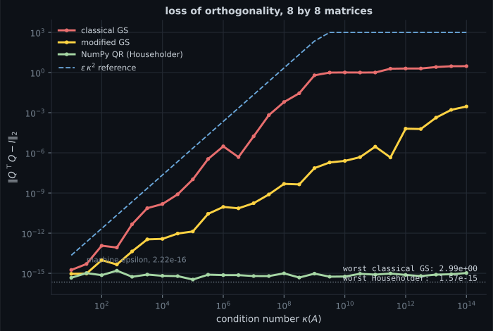
Reading the plot

From the orthogonality plot. Three things.

The classical curve tracks $\varepsilon\kappa^2$ — the dashed reference — rather than $\varepsilon\kappa$. Squaring the condition number is what forming inner products against the original columns costs you, and it is the same squaring that makes the book’s $[\tilde{\mathbf{B}}\tilde{\mathbf{B}}^\top \mid \tilde{\mathbf{B}}]$ route inadvisable in floating point: $\tilde{\mathbf{B}}\tilde{\mathbf{B}}^\top$ has the square of $\tilde{\mathbf{B}}$‘s condition number before elimination even starts.

The classical curve then saturates near $1$ and stops rising. That is not the error levelling off, it is the error running out of room: $\lVert\mathbf{Q}^\top\mathbf{Q} - \mathbf{I}\rVert$ cannot grow much past a small constant once the columns bear no relation to orthonormality. A flat tail here means total failure, not stability.

Householder is flat at the bottom, and flat for a different reason: it never forms an inner product between two nearly-parallel columns. It builds $\mathbf{Q}$ as a product of reflections, each of which is exactly orthogonal by construction, so the orthogonality of the result does not depend on the conditioning of the input at all.

From the Parseval bars. Both panels report a reconstruction error at machine precision, which is the control: both bases genuinely represent the vector, and neither expansion is wrong. What differs is whether the coordinates are interpretable. Under the ONB the squared coordinates sum to $5.845617$, which is $\lVert\mathbf{x}\rVert^2$ to within $8.88\times10^{-16}$. Under the skewed basis they sum to $11.526946$ — nearly double — so any statement of the form “this component accounts for $30\%$ of the energy” is meaningless in that basis. The skewed basis here has condition number only $6.79$, which is mild; the failure is not a numerical one, it is that Parseval simply is not true off an ONB.

That is the property PCA’s variance-explained percentages rest on, and it is why they are quoted for principal components and never for the columns of an arbitrary factor loading matrix.

Pitfalls

Do not implement classical Gram-Schmidt

The measurement is on this page: at $\kappa = 10^{10}$ it returns columns that are not orthonormal in any useful sense. If you need an orthonormal basis, call np.linalg.qr. If you need it incrementally — one vector at a time, which QR does not offer — use modified Gram-Schmidt with reorthogonalisation (run the subtraction loop twice), which recovers machine precision at roughly double the cost.

np.linalg.qr gives you an orthonormal basis, not the one you had in mind

The signs of $\mathbf{Q}$‘s columns are whatever the Householder reflections produce, not a convention you can rely on; measured, np.linalg.qr returns $\det\mathbf{Q} = (-1)^{n-1}$ for square input, so it is a reflection in every even dimension. If your output depends on the sign — a PCA loading plot, a saved model, a regression test — fix it yourself, conventionally by forcing the largest-magnitude entry of each column to be positive.

Orthogonal is not orthonormal, and the projection formula cares

A basis satisfying only Equation 3.33 has $\mathbf{B}^\top\mathbf{B}$ diagonal but not the identity, so $\boldsymbol{\lambda} = \mathbf{B}^\top\mathbf{x}$ is wrong by a factor of $\lVert\mathbf{b}_i\rVert^2$ per coordinate. The fix is to divide: $\lambda_i = \langle\mathbf{b}_i,\mathbf{x}\rangle / \langle\mathbf{b}_i,\mathbf{b}_i\rangle$. The Gram-Schmidt formula above has exactly this division in it for exactly this reason.

Gram-Schmidt’s output depends on the input order

$\mathbf{u}_1$ is $\mathbf{b}_1$ unchanged, so the first vector you list is the one that survives. A different ordering gives a genuinely different ONB of the same subspace. This is fine mathematically and a nuisance in practice: shuffle your columns and your “first basis direction” changes, even though the span and the projection onto it do not.

Orthonormality is relative to an inner product, like everything else here

$\mathbf{B}^\top\mathbf{B} = \mathbf{I}$ tests orthonormality under the dot product. Under a general inner product with matrix $\mathbf{A}$, the test is $\mathbf{B}^\top\mathbf{A}\mathbf{B} = \mathbf{I}$, and a basis orthonormal under one is generally not orthonormal under the other. There is a worked case of this in the Inner Products exercises, where $(1,0)$ and $(1,1)$ turn out to be orthonormal under the book’s Example 3.3.

Compare

basis type	Gram matrix $\mathbf{B}^\top\mathbf{B}$	coordinates of $\mathbf{x}$	cost	Parseval?
general	full, symmetric positive definite	$(\mathbf{B}^\top\mathbf{B})^{-1}\mathbf{B}^\top\mathbf{x}$	$O(n^3)$ solve	no
orthogonal	diagonal	$\langle\mathbf{b}_i,\mathbf{x}\rangle / \lVert\mathbf{b}_i\rVert^2$	$O(n^2)$, no solve	with weights
orthonormal	$\mathbf{I}$	$\langle\mathbf{b}_i,\mathbf{x}\rangle$	$O(n^2)$, no solve	yes

pch.quizTag Check your understanding

1. What does an orthonormal basis buy you that a general basis does not?

   A It spans a larger subspace B Coordinates become independent inner products rather than the solution of a system, so adding a new orthonormal direction leaves every earlier coordinate untouched — which is what makes truncation graceful C It is unique D It always has smaller entries
   pch.quizShowAnswer

   B — Coordinates become independent inner products rather than the solution of a system, so adding a new orthonormal direction leaves every earlier coordinate untouched — which is what makes truncation graceful — It is not unique — Gram-Schmidt's answer depends on the input order, and QR's column signs are arbitrary. The span is identical by construction. What changes is that B-transpose B is the identity, so the middle factor of the coordinate formula disappears.

2. Classical Gram-Schmidt at condition number 1e10 gives ||Q-transpose Q minus I|| = 1.013. What does that number mean?

   A The columns are orthonormal to about one percent B Orthogonality is completely gone — the identity matrix itself has 2-norm 1, so an error of 1.013 is the same size as the thing being approximated C The matrix was singular D The tolerance was set too tightly
   pch.quizShowAnswer

   B — Orthogonality is completely gone — the identity matrix itself has 2-norm 1, so an error of 1.013 is the same size as the thing being approximated — At 1e14 it reaches 2.993, three times the norm of the identity. The curve saturating near 1 is the error running out of room rather than levelling off. Householder QR on the same matrices never exceeds 1.052e-15.

3. Parseval's identity fails for the skewed basis in the figure, but that basis reconstructs the vector to machine precision. What is the lesson?

   A The skewed basis is not a basis B Both expansions are correct; only the orthonormal one has coordinates whose squares are interpretable as shares of the total energy — which is why variance-explained percentages are quoted for principal components and not for arbitrary loadings C The vector was not in the subspace D The skewed basis is ill-conditioned
   pch.quizShowAnswer

   B — Both expansions are correct; only the orthonormal one has coordinates whose squares are interpretable as shares of the total energy — which is why variance-explained percentages are quoted for principal components and not for arbitrary loadings — Its condition number is 6.79, which is mild, and the reconstruction error is 2.16e-15. The failure is structural rather than numerical: the squared coordinates sum to 11.53 against a squared length of 5.85.

4. A basis satisfies only Equation 3.33 — pairwise orthogonal, but not unit length. What breaks?

   A Nothing; the two conditions are equivalent B The coordinate formula: lambda-i is the inner product divided by the squared length of the basis vector, not the plain inner product, so B-transpose x is wrong by a per-coordinate factor C Orthogonality itself D The basis no longer spans the space
   pch.quizShowAnswer

   B — The coordinate formula: lambda-i is the inner product divided by the squared length of the basis vector, not the plain inner product, so B-transpose x is wrong by a per-coordinate factor — The Gram matrix is diagonal rather than the identity, so the middle factor of the coordinate formula is a diagonal inverse rather than nothing. The division appears explicitly in the Gram-Schmidt formula for exactly this reason.

🧪 Try It Yourself

Exercise 1 – Verify Example 3.8 and use it

pch.exerciseTag pch.exerciseTitle

Exercise 2 – Gram-Schmidt on the book’s Exercise 3.8

pch.exerciseTag pch.exerciseTitle

Exercise 3 – Watch classical Gram-Schmidt fail

pch.exerciseTag pch.exerciseTitle

Exercise 4 – Break Parseval

pch.exerciseTag pch.exerciseTitle

Exercise 5 – Order matters

pch.exerciseTag pch.exerciseTitle

Recall card

• An orthonormal basis is pairwise orthogonal and unit length — Definition 3.9’s two equations, which together say the Gram matrix B-transpose B is the identity.
• Coordinates become inner products: lambda equals B-transpose x, one independent inner product per basis vector, with no system to solve.
• Adding a new orthonormal direction leaves every earlier coordinate unchanged, which is what makes truncation graceful in Fourier series, wavelets and PCA.
• Parseval’s identity holds only for an orthonormal basis: the squared coordinates add up to the squared length. Measured off an ONB the sum was 11.53 against a squared length of 5.85, on a well-conditioned basis.
• Gram-Schmidt subtracts the projection onto everything already accepted and normalises. Its output depends on the input order, because the first vector survives unchanged.
• Do not implement classical Gram-Schmidt. At condition number ten to the tenth it returns columns that are not orthonormal at all; modified Gram-Schmidt is seven orders better and Householder QR never leaves machine precision.
• Forming B-transpose B squares the condition number, which is why both classical Gram-Schmidt and the augmented-matrix route lose accuracy where a Householder factorisation does not.
• The projection formula collapses to B B-transpose for an orthonormal basis, and that collapse is what section 3.8 spends most of its time earning.

Next: Orthogonal Complement — what happens to everything the basis misses.