Fine-Tuning and Parameter-Efficient Tuning (LoRA)

Transfer learning asked whether pretrained weights help. This page asks a narrower and more practical question: given that you are going to adapt a pretrained model, which weights do you actually update, and what does each answer cost?

The interesting answer is LoRA — freeze the pretrained matrix entirely and learn a small low-rank correction beside it. It is how most large models are adapted in practice, and the mechanism is simple enough to implement in about twenty lines.

What you’ll learn

The four places you can put your trainable parameters, and what each is worth.
LoRA derived and implemented: $W + BA$ , why $B$ starts at zero, what the rank buys.
The measured trade: 0.8911 from 7,493 parameters against 0.9385 from 268,037.
Why LoRA’s real argument is storage per task, not accuracy.
Why, on this task, training from scratch beat both frozen strategies — and what that tells you about when adaptation is worth anything at all.

The base model and the four strategies

A 784 → 256 → 256 → 5 network, 268,037 parameters, pretrained on Fashion-MNIST classes 0–4 to 0.8696 in 7.7 seconds. The target task is classes 5–9 with only 1,500 training rows, twelve epochs, everything averaged over two seeds.

Strategy	What trains
From scratch	Everything, no pretrained weights at all. The floor.
Frozen features + head	Both hidden layers frozen; only the new 5-way head.
Unfreeze last hidden	Second hidden layer plus the head.
LoRA rank 4	Both hidden layers frozen; a rank-4 correction on each, plus the head.
Full fine-tune	Everything, starting from the pretrained weights.

Left: horizontal bars of target accuracy for five strategies — from scratch 0.9350, frozen features 0.7605, unfreeze last hidden 0.9071, LoRA rank 4 0.8911, full fine-tune 0.9385. Right: the same accuracies plotted against trainable parameters on a log axis, showing frozen features far left at low accuracy, LoRA in the middle, and the two full-parameter strategies at the right. — The right panel is the one to read. Accuracy rises with trainable parameters but not proportionally: LoRA spends 2.8% of the parameters to get within 0.0474 of full fine-tuning, while frozen features spend 0.48% and fall 0.1780 short. Note where 'from scratch' sits — at 0.9350 it beats every strategy that froze anything, which is a fact about this task rather than about the methods.

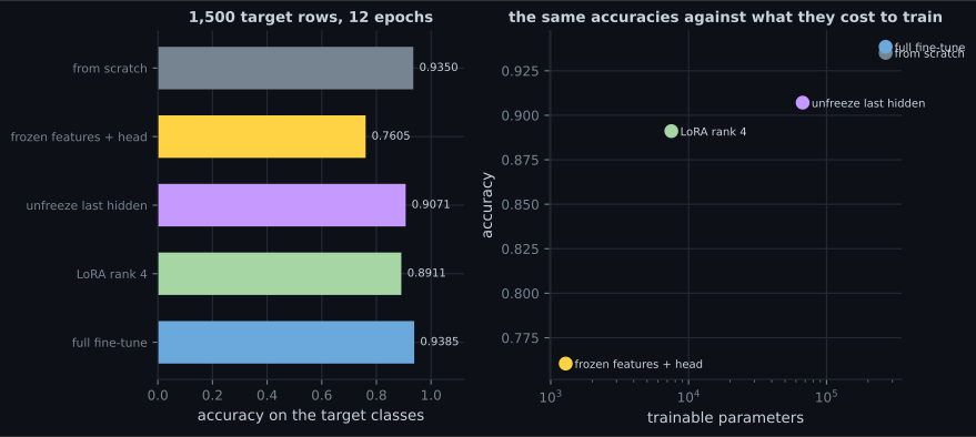
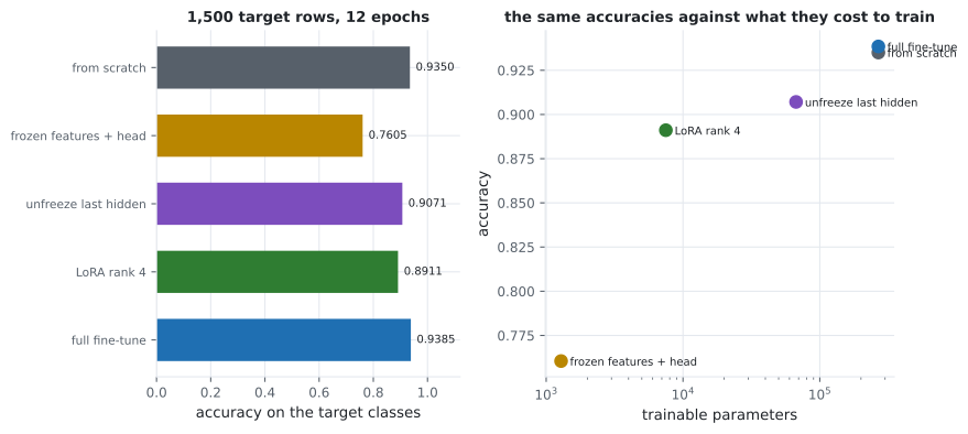
Strategy	Accuracy	Seed spread	Trainable	Share of model	Seconds
From scratch	0.9350	0.0053	268,037	100%	3.3
Frozen features + head	0.7605	0.0846	1,285	0.48%	4.3
Unfreeze last hidden	0.9071	0.0117	67,077	25.0%	2.9
LoRA rank 4	0.8911	0.0057	7,493	2.80%	3.1
Full fine-tune	0.9385	0.0032	268,037	100%	5.6

The result that has to be reported first

Training from scratch scored 0.9350 — higher than LoRA, higher than the linear probe, and within 0.0035 of full fine-tuning. Every adaptation strategy that froze weights did worse than not using the pretrained model at all.

That is not a failure of LoRA. It is a statement about when adaptation is worth anything:

The target task is easy and there is enough data for it. 1,500 rows of Fashion-MNIST footwear and bags is plenty for a 268k-parameter MLP. Adaptation methods earn their keep when target data is scarce relative to the model.
The base task is small. Features learned from five garment classes are not a rich general-purpose representation. There is little to transfer, so freezing costs more than it saves.
The frozen-feature spread is 0.0846 — sixteen times the full fine-tune’s 0.0032. When only a 1,285-parameter head trains, the outcome depends heavily on whether the frozen features happen to suit the new labels, and on this seed pair they sometimes did not.

At the scale where LoRA is actually used — a base model pretrained on far more data than the target task has, and a target set of a few thousand examples — the ordering reverses. This page cannot demonstrate that, and says so rather than picking a configuration that would flatter the method.

LoRA, derived

Full fine-tuning updates $W \in \mathbb{R}^{d \times k}$ directly, producing a whole new matrix per task. LoRA keeps $W$ frozen and learns an update constrained to be low rank:

W' = W + \Delta W, \qquad \Delta W = BA, \qquad B \in \mathbb{R}^{d \times r},\; A \in \mathbb{R}^{r \times k},\; r \ll \min(d, k)

The forward pass becomes

\mathbf{y} = \mathbf{x}W + \mathbf{x}BA + \mathbf{b}

and the parameter count drops from $dk$ to $r(d + k)$ . For the 256×256 layers here at $r = 4$ : 65,536 → 2,048, a 32× reduction per matrix.

Two implementation details carry the whole method:

$B$ is initialised to zero. Then $\Delta W = BA = 0$ at step one, so the wrapped layer is numerically identical to the frozen one before any training happens. Adaptation starts from the pretrained function exactly, with no random perturbation to recover from. Initialising both factors randomly would inject noise into a model you just paid to pretrain.

Only $A$ and $B$ receive gradients. $W$ is frozen, so the optimiser state — Adam keeps two moments per trainable parameter — also shrinks by the same factor. On a large model that optimiser state is usually the memory that actually stops you.

python

class LoRADense(keras.layers.Layer):
    def __init__(self, base, rank, **kwargs):
        super().__init__(**kwargs)
        self.base = base
        self.base.trainable = False          # W never moves
        self.rank = rank
 
    def build(self, shape):
        inputs = int(self.base.kernel.shape[0])
        outputs = int(self.base.kernel.shape[1])
        self.down = self.add_weight(shape=(inputs, self.rank),
                                    initializer="glorot_uniform")
        self.up = self.add_weight(shape=(self.rank, outputs),
                                  initializer="zeros")      # B starts at 0
 
    def call(self, x):
        correction = tf.matmul(tf.matmul(x, self.down), self.up)
        return self.base.activation(
            tf.matmul(x, self.base.kernel) + self.base.bias + correction)

diagram Diagram mermaid

  flowchart LR
  X["x"] --> W["frozen W
65,536 weights"]
  X --> A["A: 256 x r
trainable"]
  A --> B["B: r x 256
trainable, starts at 0"]
  W --> S["+"]
  B --> S
  S --> Y["y"]
  W -.->|"never updated,
no optimiser state"| N["shared across
every task"]

What the rank buys

Rank is the only knob LoRA exposes. It is the inner dimension of the correction, and it sets both capacity and cost:

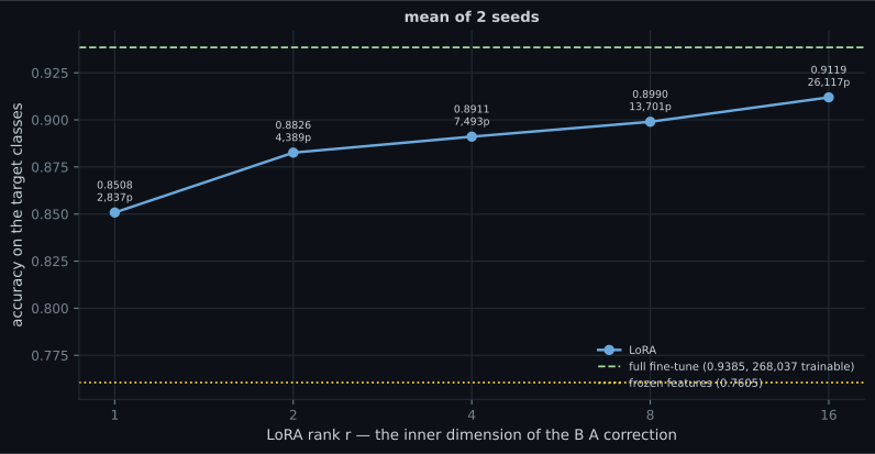
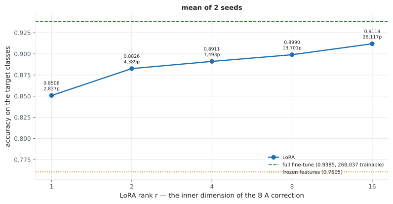
Accuracy against LoRA rank on a log-2 axis, rising from 0.8508 at rank 1 to 0.9119 at rank 16, each point annotated with its trainable parameter count from 2,837 to 26,117. A dashed line marks full fine-tuning at 0.9385 and a dotted line marks frozen features at 0.7605. — Monotone but flattening. Rank 1 already reaches 0.8508 — well above the 0.7605 of a frozen-feature probe with a comparable-order parameter count — and doubling the rank four times buys 0.0611 more. Every point sits between the two dashed lines, which is the honest summary of the method: strictly better than freezing, strictly worse than updating everything, at a cost you choose.

Rank $r$	Accuracy	Trainable	Against full fine-tune
1	0.8508	2,837	−0.0877
2	0.8826	4,389	−0.0559
4	0.8911	7,493	−0.0474
8	0.8990	13,701	−0.0395
16	0.9119	26,117	−0.0266

Doubling the rank roughly doubles the trainable parameters and buys progressively less: +0.0318 from rank 1 to 2, then +0.0085, +0.0079, +0.0129. There is no cliff and no sweet spot — just a dial between “cheap” and “close to full fine-tuning”.

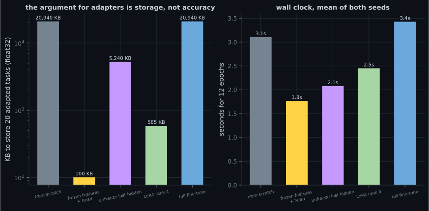
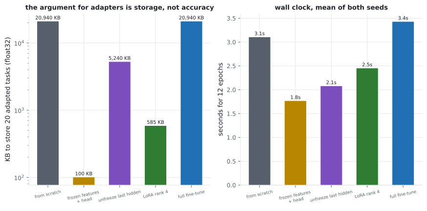
The argument that actually matters

LoRA does not win on accuracy. It wins on what you keep afterwards.

figure Twenty tasks adapted from one base model, float32 matplotlib

Full fine-tuning stores an entire 268,037-parameter model per task — 20,940 KB for twenty tasks. LoRA stores 7,493 numbers per task and shares the frozen base: 585 KB, a 35.8x reduction, for 0.0474 less accuracy. The right panel shows what the method does NOT buy at this scale: wall clock is dominated by the forward pass, which is unchanged, so training time barely moves.

Strategy	Per task	20 tasks	Accuracy cost
Full fine-tune	1,047 KB	20,940 KB	—
Unfreeze last hidden	262 KB	5,240 KB	−0.0314
LoRA rank 4	29 KB	585 KB	−0.0474
Frozen features + head	5 KB	100 KB	−0.1780

Twenty task-specific models at full fine-tuning is twenty complete copies. With LoRA it is one frozen base plus twenty 29 KB adapters, and swapping tasks means swapping a 29 KB file. Multiply by a real base model and this is the difference between one deployment and twenty.

Note what it does not buy here. Wall clock moved from 5.6 s to 3.1 s, and that is mostly noise on runs this short — the forward pass through the frozen weights costs the same either way, and LoRA adds two small matrix multiplies to it. Parameter-efficient tuning saves memory and storage, not arithmetic. On a large model the memory saving is what lets the run happen at all, but the per-step compute is roughly unchanged.

sketch Where the parameters go p5.js

Drag to set the LoRA rank. The bars show the measured accuracy and the trainable parameter count against the two reference lines.

sketch The measured table, ranked p5.js

Click a column to rank every row by it. The bars are that column's values and the highest and lowest are computed from the numbers, not written in.

Pitfalls

Reporting LoRA without a from-scratch baseline. Here scratch scored 0.9350 and beat it. Without that row the page would read as an endorsement it has not earned.
Initialising $B$ randomly. With $B = 0$ the adapted model starts exactly at the pretrained function. Random initialisation on both factors injects noise into weights you paid to pretrain.
Expecting a speed-up. Wall clock barely moved. LoRA cuts trainable parameters, optimiser state and stored bytes — not the forward pass.
Judging a frozen-feature probe on one seed. Its spread across two seeds was 0.0846 against full fine-tuning’s 0.0032; a single run could land anywhere in that band.
Choosing the rank by accuracy alone. The curve is monotone, so accuracy alone always says “higher”. The question is what accuracy per stored kilobyte you need.
Assuming these numbers transfer to a large base model. They do not, and in a specific direction: the case for adaptation gets stronger as the base model grows and the target set shrinks.

Recap

The base model — 268,037 parameters, pretrained to 0.8696 on classes 0–4 — was adapted to classes 5–9 with 1,500 rows, five ways.
LoRA rank 4 reached 0.8911 while training 7,493 parameters, 2.80% of the model — 35.8× fewer than full fine-tuning’s 0.9385.
The rank sweep is monotone and flattening: 0.8508 at $r=1$ through 0.9119 at $r=16$ , every point strictly between a frozen probe and full fine-tuning.
The real argument is storage: 585 KB for twenty adapted tasks against 20,940 KB. Wall clock barely moved, because the forward pass is unchanged.
$B$ initialised to zero is what lets adaptation start from the pretrained function exactly.
Training from scratch scored 0.9350 and beat every frozen strategy, because the target task had enough data and the base task was small. Adaptation methods are worth their complexity when target data is scarce relative to the model — which is a condition to check, not to assume.

Data Augmentation for Small Datasets — the other standard answer to “not enough target data”, and one that also costs accuracy on the distribution you measured.

pch.quizTag pch.quizDefaultTitle

Training from scratch scored 0.9350 while LoRA scored 0.8911 and a frozen-feature probe 0.7605. What is the correct reading?

pch.quizShowAnswer

B — Adaptation pays when target data is scarce relative to the model; here 1,500 rows was plenty and the base task (five garment classes) was too small to have learned much worth transferring
In LoRA, why is B initialised to zero rather than randomly?

pch.quizShowAnswer

B — So that BA = 0 at step one and the wrapped layer is numerically identical to the frozen pretrained layer — adaptation starts from the pretrained function with no noise to recover from
LoRA reduced trainable parameters 35.8x but wall clock moved only 5.6 s to 3.1 s. Why so little?

pch.quizShowAnswer

B — LoRA saves memory, optimiser state and stored bytes - the forward pass still runs through the full frozen matrix, and LoRA adds two small multiplies on top of it
The frozen-feature probe's accuracy varied by 0.0846 across two seeds while full fine-tuning varied by 0.0032. What causes the difference?

pch.quizShowAnswer

B — With only a 1,285-parameter head trainable, the result depends almost entirely on whether the fixed features happen to suit the new labels - there is no capacity to compensate when they do not
For a 256x256 weight matrix at rank 4, LoRA replaces 65,536 trainable numbers with how many, and by what formula?

pch.quizShowAnswer

B — 2,048, from r(d + k) = 4 x (256 + 256)
The rank sweep rose monotonically from 0.8508 to 0.9119. Why is 'pick the highest rank' still the wrong default?

pch.quizShowAnswer

B — Because the curve flattens while cost keeps doubling - the decision is accuracy per stored kilobyte, and rank 16 costs 3.5x rank 4's storage for 0.0208 more accuracy

🧪 Try It Yourself

pch.coffeeTagline

pch.coffeeCta

pch.feedbackHeading

pch.feedbackSubheading