Constrained Optimization and Lagrange Multipliers

Everything so far assumed the answer could be anywhere. It usually cannot. A probability must stay in $[0,1]$, a portfolio’s weights must sum to one, an SVM’s margin variables must stay non-negative (Chapter 12). So:

$$\min_{\mathbf{x}} f(\mathbf{x}) \qquad\text{subject to}\qquad g_i(\mathbf{x}) \leq 0 \quad\text{for all } i = 1, \dots, m$$

The trouble is that gradient descent has no idea what a constraint is. This page is the standard way to teach it one, and the move is smaller than it looks: replace an infinite wall with a slope.

What you’ll learn

• Equations 7.18 and 7.19: the indicator-function reformulation, which is exactly correct and completely unoptimisable — measured, its gradient is undefined everywhere outside the feasible set.
• Equation 7.20, the Lagrangian, and why a linear penalty is the right relaxation.
• Definition 7.1: the primal problem, the dual problem, and $D(\boldsymbol\lambda) = \min_{\mathbf{x}} L(\mathbf{x}, \boldsymbol\lambda)$.
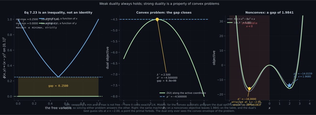
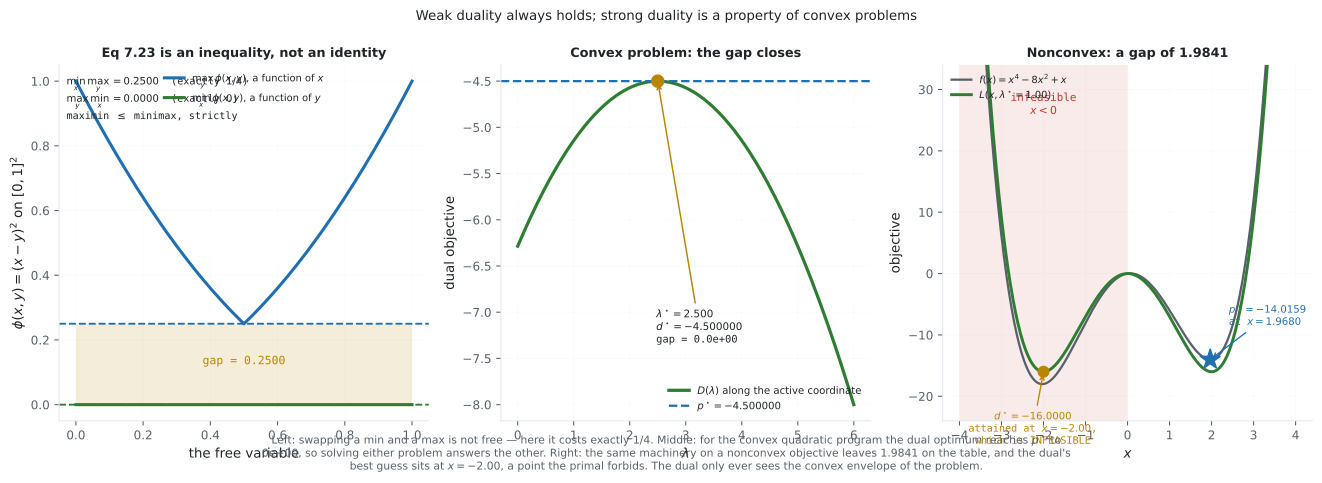
• The minimax inequality (Equation 7.23) with a worked case where the gap is exactly $1/4$, so you can see it is an inequality rather than an identity.
• Weak duality (Equation 7.27), and why the dual is always concave even when the primal is a mess.
• Measured on the book’s Example 7.6: $\lambda^\star = 2.5$, duality gap exactly zero, and complementary slackness holding to machine precision.
• Measured on a nonconvex problem: a duality gap of 1.984123, with the dual’s optimum attained at $x = -2$, a point the primal forbids.
• Equation 7.28: how equality constraints fold in, and why their multipliers come out unconstrained.

Intuition: a wall you can feel, or a wall you cannot

You are minimising altitude, and there is a fence.

The naive fix is to declare the far side of the fence infinitely high. That is honest — you will never end up there — but it is useless to a hiker in fog. Step over the fence and everything reads “infinitely high”, in every direction. Nothing tells you which way to go back.

The Lagrangian fix is to charge rent instead. Crossing the fence by one metre costs $\lambda$ altitude-units. Now the far side is still discouraging, but it has a slope, and a slope is the one thing a gradient method can use. Better still, you get to pick $\lambda$: too small and the optimum sits outside the fence, too large and it hugs the fence unnecessarily. Somewhere in between is a price at which the unconstrained optimum of the rented landscape lands exactly on the fence — and that price is $\lambda^\star$.

diagram From an unoptimisable reformulation to a solvable one mermaid

  flowchart TD
  P["primal, Eq 7.17
min f subject to g <= 0"]
  P --> I["Eq 7.18: add an indicator
J = f + sum of 1(g_i)"]
  I --> BAD["exactly equivalent
but +infinity everywhere outside:
no gradient, no method"]
  P --> LAG["Eq 7.20: add lambda-transpose g
a LINEAR penalty"]
  LAG --> SMOOTH["smooth in x for fixed lambda,
and a lower bound for lambda >= 0"]
  SMOOTH --> D["Eq 7.22: the dual
max over lambda of min over x"]
  D --> CONC["always CONCAVE in lambda,
however ugly f and g are"]
  CONC --> W["Eq 7.27: weak duality
d-star <= p-star, always"]
  W --> S["convex primal: gap is ZERO
Section 7.3"]
  W --> G["nonconvex primal: gap can be real
measured 1.984123"]

The math

First attempt: an indicator function

Turn the constraint into a penalty that is free when satisfied and unbearable when not:

$$J(\mathbf{x}) = f(\mathbf{x}) + \sum_{i=1}^{m}\mathbf{1}\big(g_i(\mathbf{x})\big), \qquad \mathbf{1}(z) = \begin{cases} 0 & \text{if } z \leq 0\\ \infty & \text{otherwise}\end{cases}$$

Minimising $J$ over all of $\mathbb{R}^D$ gives exactly the constrained answer, because any infeasible point scores $+\infty$. So this reformulation is correct. It is also, in the book’s words, “equally difficult to optimize”, and it is worth being precise about why: the penalty is not merely steep, it is flat at infinity. Every infeasible point looks identical to every other one, so a gradient computed out there is undefined and carries no information about the direction of the feasible set. There is nothing to descend.

Second attempt: charge linearly

Introduce Lagrange multipliers $\lambda_i \geq 0$, one per inequality, and replace the step function with a linear function:

$$L(\mathbf{x}, \boldsymbol\lambda) = f(\mathbf{x}) + \sum_{i=1}^{m}\lambda_i g_i(\mathbf{x}) = f(\mathbf{x}) + \boldsymbol\lambda^\top\mathbf{g}(\mathbf{x})$$

stacking the constraints into $\mathbf{g}(\mathbf{x})$ and the multipliers into $\boldsymbol\lambda \in \mathbb{R}^m$.

Two properties, and everything else on this page follows from them:

• For $\boldsymbol\lambda \geq 0$ and $\mathbf{x}$ feasible, $L(\mathbf{x}, \boldsymbol\lambda) \leq f(\mathbf{x})$. Each $g_i(\mathbf{x}) \leq 0$ and each $\lambda_i \geq 0$, so every term in the sum is non-positive. The Lagrangian under-estimates the objective on the feasible set.
• Taking the maximum over $\boldsymbol\lambda$ recovers the indicator exactly. $$J(\mathbf{x}) = \max_{\boldsymbol\lambda \geq 0} L(\mathbf{x}, \boldsymbol\lambda)$$ If $\mathbf{x}$ is feasible, the best you can do is set $\boldsymbol\lambda = \mathbf{0}$ and get $f(\mathbf{x})$. If some $g_i(\mathbf{x}) > 0$, push that $\lambda_i \to \infty$ and the supremum is $+\infty$. The infinite step function has been reconstructed as a maximum of linear functions, which is the actual trick.

So the original problem is

$$\min_{\mathbf{x}\in\mathbb{R}^d} \max_{\boldsymbol\lambda \geq 0} L(\mathbf{x}, \boldsymbol\lambda)$$

Definition 7.1: primal and dual

The primal problem is the one we started with, in the variables $\mathbf{x}$. Its Lagrangian dual problem is

$$\max_{\boldsymbol\lambda\in\mathbb{R}^m} D(\boldsymbol\lambda) \qquad\text{subject to}\qquad \boldsymbol\lambda \geq 0, \qquad\text{where } D(\boldsymbol\lambda) = \min_{\mathbf{x}\in\mathbb{R}^d} L(\mathbf{x}, \boldsymbol\lambda)$$

Duality in general means converting a problem in one set of variables into a problem in another. Note what has been traded: the primal has $d$ variables and $m$ constraints; the dual has $m$ variables and the single requirement $\boldsymbol\lambda \geq 0$. If $m \ll d$ that is a bargain, and §7.3.1 makes the choice explicit for linear programs.

The minimax inequality

For any function of two arguments,

$$\max_{\mathbf{y}} \min_{\mathbf{x}} \phi(\mathbf{x}, \mathbf{y}) \;\leq\; \min_{\mathbf{x}} \max_{\mathbf{y}} \phi(\mathbf{x}, \mathbf{y})$$

Maximin is at most minimax. The proof is two lines. Start from the observation that for all $\mathbf{x}, \mathbf{y}$,

$$\min_{\mathbf{x}} \phi(\mathbf{x}, \mathbf{y}) \;\leq\; \max_{\mathbf{y}} \phi(\mathbf{x}, \mathbf{y})$$

The left side does not depend on $\mathbf{x}$ and the right side does not depend on $\mathbf{y}$, so take the maximum over $\mathbf{y}$ on the left — legitimate, since the inequality holds for every $\mathbf{y}$ — and the minimum over $\mathbf{x}$ on the right. The inequality survives both, giving the result.

The intuition worth keeping: the player who moves second has the advantage. On the minimax side $\mathbf{y}$ sees $\mathbf{x}$ before choosing; on the maximin side $\mathbf{x}$ sees $\mathbf{y}$. Whoever reacts does at least as well.

Weak duality

Apply that to the Lagrangian:

$$\min_{\mathbf{x}\in\mathbb{R}^d} \max_{\boldsymbol\lambda \geq 0} L(\mathbf{x}, \boldsymbol\lambda) \;\geq\; \max_{\boldsymbol\lambda \geq 0} \min_{\mathbf{x}\in\mathbb{R}^d} L(\mathbf{x}, \boldsymbol\lambda)$$

The left side is the primal optimum $p^\star$; the right side is the dual optimum $d^\star$. So $d^\star \leq p^\star$, always — that is weak duality, and it means any dual feasible $\boldsymbol\lambda$ hands you a certified lower bound on the primal answer, for free.

The dual is concave even when the primal is horrible

$D(\boldsymbol\lambda) = \min_{\mathbf{x}} L(\mathbf{x}, \boldsymbol\lambda)$ is, for each fixed $\mathbf{x}$, an affine function of $\boldsymbol\lambda$. A pointwise minimum of affine functions is concave. So $D$ is concave no matter how nonconvex $f$ and the $g_i$ are — and maximising a concave function is easy. The book makes exactly this point: “the outer problem is a maximum over a set of affine functions, and hence is a concave function, even though $f(\cdot)$ and $g_i(\cdot)$ may be nonconvex.”

That is the real payoff of duality. You can always get a tractable lower bound. Whether it is tight is a separate question, answered in §7.3.

Equality constraints

$$\min_{\mathbf{x}} f(\mathbf{x}) \quad\text{s.t.}\quad g_i(\mathbf{x}) \leq 0 \;\; \forall i, \qquad h_j(\mathbf{x}) = 0 \;\; \forall j$$

Each equality $h_j(\mathbf{x}) = 0$ splits into the pair $h_j(\mathbf{x}) \leq 0$ and $-h_j(\mathbf{x}) \leq 0$. Both get non-negative multipliers, say $\lambda_j^{+}$ and $\lambda_j^{-}$, and their contribution is $\lambda_j^{+}h_j - \lambda_j^{-}h_j = (\lambda_j^{+} - \lambda_j^{-})h_j$. The difference of two non-negative numbers is an arbitrary real number, so:

Inequality multipliers are constrained to be non-negative; equality multipliers are unconstrained. That asymmetry is not a convention, it is a consequence — and it is a fast way to check that you have written a Lagrangian correctly.

Worked example by hand

The book’s Example 7.6, which is also its Figure 7.4:

$$\min_{\mathbf{x}\in\mathbb{R}^2} \frac{1}{2}\begin{bmatrix}x_1\\x_2\end{bmatrix}^\top\begin{bmatrix}2&1\\1&4\end{bmatrix}\begin{bmatrix}x_1\\x_2\end{bmatrix} + \begin{bmatrix}5\\3\end{bmatrix}^\top\begin{bmatrix}x_1\\x_2\end{bmatrix}$$

subject to $-1 \leq x_1 \leq 1$ and $-1 \leq x_2 \leq 1$, written in the standard form $\mathbf{A}\mathbf{x} \leq \mathbf{b}$ with

$$\mathbf{A} = \begin{bmatrix}1&0\\-1&0\\0&1\\0&-1\end{bmatrix}, \qquad \mathbf{b} = \begin{bmatrix}1\\1\\1\\1\end{bmatrix}$$

Step 1: ignore the constraints. With $f = \tfrac12\mathbf{x}^\top\mathbf{Q}\mathbf{x} + \mathbf{c}^\top\mathbf{x}$ the gradient is $\mathbf{Q}\mathbf{x} + \mathbf{c}$, zero at $\mathbf{x} = -\mathbf{Q}^{-1}\mathbf{c}$. Since $\det\mathbf{Q} = 8 - 1 = 7$,

$$\mathbf{x}_{\text{unc}} = -\frac{1}{7}\begin{bmatrix}4&-1\\-1&2\end{bmatrix}\begin{bmatrix}5\\3\end{bmatrix} = -\frac{1}{7}\begin{bmatrix}17\\1\end{bmatrix} = \begin{bmatrix}-2.428571\\-0.142857\end{bmatrix}$$

with $f = -6.285714$. This point is infeasible: $x_1 = -2.43$ violates $x_1 \geq -1$ by $1.428571$.

Step 2: the constraint must bind. Since the objective is a strictly convex bowl and its centre lies outside the box, the constrained optimum sits on the boundary — on the face nearest the centre, which is $x_1 = -1$. Substituting:

$$f(-1, x_2) = \tfrac12\big(2 - 2x_2 + 4x_2^2\big) - 5 + 3x_2 = 2x_2^2 + 2x_2 - 4$$

A one-variable quadratic. Its derivative $4x_2 + 2$ vanishes at $x_2 = -\tfrac12$, comfortably inside $[-1,1]$, giving

$$\mathbf{x}^\star = \begin{bmatrix}-1\\-1/2\end{bmatrix}, \qquad f(\mathbf{x}^\star) = 2\cdot\tfrac14 - 1 - 4 = -4.5$$

So the constraint costs $-4.5 - (-6.285714) = 1.785714$ in objective value.

Step 3: read off the multipliers. At a constrained optimum the stationarity condition is $\mathbf{Q}\mathbf{x}^\star + \mathbf{c} + \mathbf{A}^\top\boldsymbol\lambda^\star = \mathbf{0}$.

$$\mathbf{Q}\mathbf{x}^\star + \mathbf{c} = \begin{bmatrix}2(-1) + 1(-\tfrac12)\\1(-1) + 4(-\tfrac12)\end{bmatrix} + \begin{bmatrix}5\\3\end{bmatrix} = \begin{bmatrix}-2.5\\-3\end{bmatrix} + \begin{bmatrix}5\\3\end{bmatrix} = \begin{bmatrix}2.5\\0\end{bmatrix}$$

Only the second row of $\mathbf{A}$ (the constraint $-x_1 \leq 1$) is active, and $\mathbf{A}^\top\boldsymbol\lambda = \lambda_2\begin{bmatrix}-1\\0\end{bmatrix}$. So we need $2.5 - \lambda_2 = 0$:

$$\boldsymbol\lambda^\star = \begin{bmatrix}0\\2.5\\0\\0\end{bmatrix}$$

Notice that the second component of $\mathbf{Q}\mathbf{x}^\star + \mathbf{c}$ came out exactly zero. That is not luck: $x_2$ is interior, so no constraint pushes on it, so $f$ must already be flat in that direction. Constrained optimality is “flat where you are free, pushed where you are pinned”.

Step 4: complementary slackness. For each $i$, either $g_i(\mathbf{x}^\star) = 0$ or $\lambda_i^\star = 0$:

$i$	constraint	$g_i(\mathbf{x}^\star)$	$\lambda_i^\star$	product	status
1	$x_1 \leq 1$	$-2$	$0$	$0$	slack
2	$-x_1 \leq 1$	$\mathbf{0}$	$\mathbf{2.5}$	$0$	active
3	$x_2 \leq 1$	$-1.5$	$0$	$0$	slack
4	$-x_2 \leq 1$	$-0.5$	$0$	$0$	slack

A multiplier is the price of a constraint. A constraint that is not binding is free.

A note on the book’s Figure 7.4 caption

The caption states that the unconstrained problem “has a minimum on the right side”. Computing Equation 7.46 exactly as printed — with $+\mathbf{c}^\top\mathbf{x}$ and $\mathbf{c} = [5,3]^\top$ — puts the unconstrained minimum at $(-17/7, -1/7) \approx (-2.43, -0.14)$, which is on the left. The phrasing matches Figure 7.9’s caption, where for the linear program of Equation 7.44 the objective is $-[5,3]^\top\mathbf{x}$ and the minimum genuinely is up and to the right. Nothing downstream depends on this, and the mathematics of Example 7.6 is unaffected — but if you are reading the two figures side by side, the sign is worth checking yourself.

See it move

The single most useful thing to feel here is $\lambda$ as a price. Drag it and watch the unconstrained minimiser of the Lagrangian walk toward the boundary; the price at which it arrives is $\lambda^\star$.

sketch A Lagrange multiplier is a price, and lambda-star is the market rate p5.js Pause Restart

The objective is Example 7.6 sliced at x2 = -0.5, so the picture is one-dimensional and honest. Drag lambda and watch two things: the Lagrangian tilting, and its minimiser sliding toward the constraint boundary. Below, D(lambda) is traced out, and its peak is the primal optimum.

A second sketch, for the fact that surprises people: the dual of a nonconvex problem is still concave and still gives a bound, but the bound need not be tight.

sketch Where the duality gap comes from p5.js Pause Restart

A nonconvex objective with one constraint. Drag lambda and watch the Lagrangian's minimiser jump between two wells rather than sliding. The dual can only ever see the lower envelope, so it never reports the primal answer — the shortfall is the duality gap.

From scratch

lagrange.py

import numpy as np
 
# The book's Example 7.6, which is also its Figure 7.4.
Q = np.array([[2.0, 1.0], [1.0, 4.0]])
c = np.array([5.0, 3.0])
A = np.array([[1.0, 0.0], [-1.0, 0.0], [0.0, 1.0], [0.0, -1.0]])
b = np.ones(4)                      # the box -1 <= x_i <= 1
 
def f(x):
    return 0.5 * x @ Q @ x + c @ x
 
def g(x):
    return A @ x - b                # feasible means every entry <= 0
 
# --- Equation 7.18: correct, and impossible to descend ---------------------
def J(x):
    return f(x) if np.all(g(x) <= 0) else np.inf
 
x_unc = np.linalg.solve(Q, -c)
print(f"unconstrained minimiser (-17/7, -1/7) = "
      f"[{x_unc[0]:.6f}, {x_unc[1]:.6f}]   f = {f(x_unc):.6f}")
print(f"feasible? {np.all(g(x_unc) <= 0)}   worst violation "
      f"{g(x_unc).max():+.6f}")
print(f"J at that point = {J(x_unc)}")
 
h = 1e-6
for probe in (np.array([-1.5, -0.5]), np.array([-3.0, -0.5])):
    fd = []
    for d in range(2):
        e = np.zeros(2); e[d] = h
        num = J(probe + e) - J(probe - e)
        fd.append("undefined" if not np.isfinite(num) else f"{num / (2*h):+.4f}")
    print(f"  finite-difference grad of J at {probe.tolist()}: ({fd[0]}, {fd[1]})")
print("  -> outside the box every direction looks identical. No slope to follow.")
 
# --- Equation 7.20: the Lagrangian ---------------------------------------
def L(x, lam):
    return f(x) + lam @ g(x)
 
def D(lam):
    """min over x of L. For a positive definite Q this is closed form."""
    v = c + A.T @ lam
    xs = np.linalg.solve(Q, -v)
    return 0.5 * xs @ Q @ xs + v @ xs - lam @ b, xs
 
x_con = np.array([-1.0, -0.5])      # solved by hand on the x1 = -1 edge
print(f"\nconstrained optimum [{x_con[0]}, {x_con[1]}]   f = {f(x_con):.6f}")
print(f"the constraint costs {f(x_con) - f(x_unc):.6f}")
 
print("\nfor lambda >= 0 the Lagrangian is a LOWER BOUND at any feasible x:")
for lam in (np.zeros(4), np.array([0.0, 1.0, 0.0, 0.0]), np.full(4, 0.5)):
    print(f"  lambda = {lam.tolist()}   L = {L(x_con, lam):+.6f}   "
          f"<= f = {f(x_con):+.6f}: {L(x_con, lam) <= f(x_con) + 1e-12}")
 
# --- the dual, maximised over the one coordinate that matters ------------
ts = np.linspace(0.0, 6.0, 60001)
dv = np.array([D(np.array([0.0, t, 0.0, 0.0]))[0] for t in ts])
k = int(np.argmax(dv))
lam_star = np.array([0.0, ts[k], 0.0, 0.0])
dstar, x_from_dual = D(lam_star)
print(f"\nlambda* = {np.round(lam_star, 6).tolist()}")
print(f"d* = {dstar:.9f}    p* = {f(x_con):.9f}    gap = {f(x_con) - dstar:.3e}")
print(f"x recovered from the dual = "
      f"[{x_from_dual[0]:.6f}, {x_from_dual[1]:.6f}]")
 
print("\ncomplementary slackness:")
for i, (l, gi) in enumerate(zip(lam_star, g(x_con))):
    print(f"  i={i}  lambda={l:8.5f}  g={gi:+8.5f}  product={l * gi:+.1e}   "
          f"{'ACTIVE' if abs(gi) < 1e-9 else 'slack'}")
print("stationarity ||Qx + c + A^T lambda|| =",
      f"{np.linalg.norm(Q @ x_con + c + A.T @ lam_star):.2e}")
 
# --- weak duality only, on a nonconvex primal ---------------------------
print("\n--- a nonconvex primal keeps a real gap -------------------------")
xs = np.linspace(-4.0, 4.0, 40001)
fn = xs ** 4 - 8.0 * xs ** 2 + xs
gn = -xs                             # the constraint x >= 0
p_star = fn[gn <= 0].min()
x_p = xs[gn <= 0][int(np.argmin(fn[gn <= 0]))]
lams = np.linspace(0.0, 6.0, 1201)
dn = np.array([(fn + t * gn).min() for t in lams])
kb = int(np.argmax(dn))
x_d = xs[int(np.argmin(fn + lams[kb] * gn))]
print(f"min x^4 - 8x^2 + x  subject to  x >= 0")
print(f"  p* = {p_star:.6f} at x = {x_p:.6f}")
print(f"  d* = {dn[kb]:.6f} at lambda = {lams[kb]:.4f}, attained at x = {x_d:.4f}")
print(f"  that x is feasible: {x_d >= 0}")
print(f"  duality GAP = {p_star - dn[kb]:.6f}")

text

unconstrained minimiser (-17/7, -1/7) = [-2.428571, -0.142857]   f = -6.285714
feasible? False   worst violation +1.428571
J at that point = inf
  finite-difference grad of J at [-1.5, -0.5]: (undefined, undefined)
  finite-difference grad of J at [-3.0, -0.5]: (undefined, undefined)
  -> outside the box every direction looks identical. No slope to follow.
 
constrained optimum [-1.0, -0.5]   f = -4.500000
the constraint costs 1.785714
 
for lambda >= 0 the Lagrangian is a LOWER BOUND at any feasible x:
  lambda = [0.0, 0.0, 0.0, 0.0]   L = -4.500000   <= f = -4.500000: True
  lambda = [0.0, 1.0, 0.0, 0.0]   L = -4.500000   <= f = -4.500000: True
  lambda = [0.5, 0.5, 0.5, 0.5]   L = -6.500000   <= f = -4.500000: True
 
lambda* = [0.0, 2.5, 0.0, 0.0]
d* = -4.500000000    p* = -4.500000000    gap = 0.000e+00
x recovered from the dual = [-1.000000, -0.500000]
 
complementary slackness:
  i=0  lambda= 0.00000  g=-2.00000  product=-0.0e+00   slack
  i=1  lambda= 2.50000  g=+0.00000  product=+0.0e+00   ACTIVE
  i=2  lambda= 0.00000  g=-1.50000  product=-0.0e+00   slack
  i=3  lambda= 0.00000  g=-0.50000  product=-0.0e+00   slack
stationarity ||Qx + c + A^T lambda|| = 0.00e+00
 
--- a nonconvex primal keeps a real gap -------------------------
min x^4 - 8x^2 + x  subject to  x >= 0
  p* = -14.015877 at x = 1.968000
  d* = -16.000000 at lambda = 1.0000, attained at x = -2.0000
  that x is feasible: False
  duality GAP = 1.984123

On real data

figure Replace an infinite step with a linear penalty matplotlib

The indicator reformulation is exactly correct and has no gradient to follow outside the feasible set. The Lagrangian is smooth for every lambda, and its minimiser reaches the boundary at exactly lambda star = 2.5, where D of lambda touches the primal optimum.

figure Example 7.6, computed rather than sketched matplotlib

The unconstrained minimiser violates the box by 1.428571, so the optimum is pinned on the x1 = minus 1 face at minus 1 comma minus one half. Only that constraint gets a nonzero multiplier, and the stationarity residual is exactly zero.

figure Weak duality always; strong duality only for convex problems matplotlib

Swapping a min and a max costs exactly one quarter in the left example. For the convex quadratic program the dual closes the gap to zero. For the nonconvex quartic it leaves 1.984123 on the table, and its best guess sits at x = minus 2, which the primal forbids.

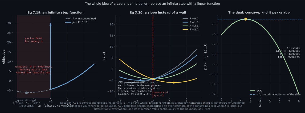
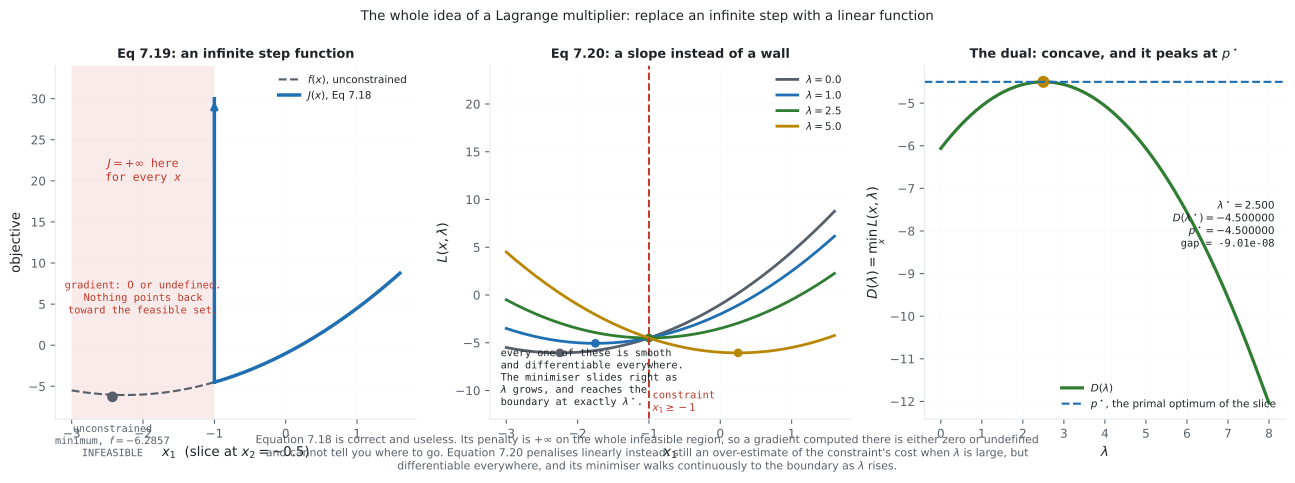
Reading the plot

The first figure is the argument of the whole page in three steps. The left panel is Equation 7.18 drawn honestly. Inside the feasible region, $J$ is $f$ — same curve, same gradient — and note which way that gradient points: out through the wall, toward the unconstrained minimum at $-2.43$. So a gradient method started anywhere feasible walks straight at the boundary and then leaves. One step past it, the value is $+\infty$ and the measured finite-difference gradient is undefined in both coordinates. Not large. Not steep. Undefined, and identically so at $x_1 = -1.5$ and at $x_1 = -3.0$. The penalty knows you have broken the rule and cannot tell you how badly.

The middle panel is the repair. Each curve is $L(x,\lambda)$ for a fixed price, and every one of them is a smooth quadratic — differentiable everywhere, no wall anywhere. Watch the marked minimisers move right as $\lambda$ grows: at $\lambda = 0$ the minimiser is the unconstrained one, and by $\lambda = 2.5$ it has arrived exactly at the boundary. The constraint has been converted from a prohibition into an incentive.

The right panel closes it. $D(\lambda)$ rises, peaks, and falls, and its peak touches the dashed line $p^\star = -4.5$ — the measured gap at the peak is $9\times10^{-8}$, which is my $\lambda$ grid resolution rather than a real shortfall. This is strong duality, and §7.3 explains why we were entitled to it: the problem is convex.

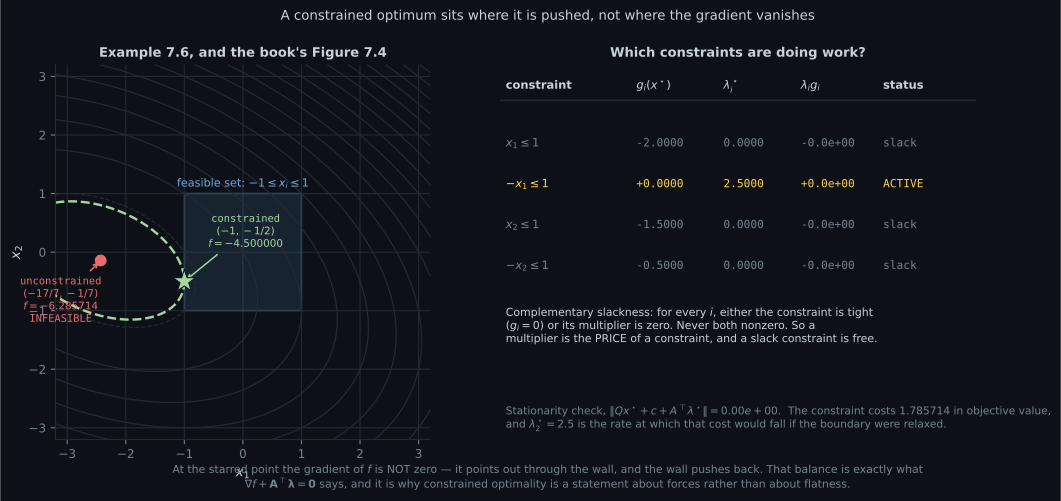
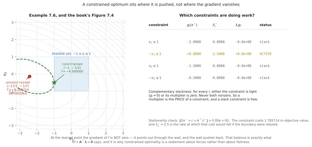
The second figure is where constrained optimality stops resembling unconstrained optimality. The red circle is where $\nabla f = \mathbf{0}$, and it is not the answer — it lies outside the box by $1.428571$. The green star is the answer, and at the green star the gradient is emphatically not zero: $\mathbf{Q}\mathbf{x}^\star + \mathbf{c} = [2.5, 0]^\top$. It points straight out through the left wall with magnitude $2.5$, and the wall pushes back with force $\lambda_2^\star = 2.5$. The condition is a balance of forces, not a vanishing derivative.

The table earns its place through the second component of that gradient: exactly $0$. The variable $x_2$ is interior — nothing is pinning it — so $f$ must already be flat along it. That is the general shape of a constrained optimum: flat in the directions you are free to move, pushed in the directions you are pinned. And complementary slackness is the bookkeeping for that: three of four constraints are slack and carry multiplier zero, one is active and carries $2.5$. A multiplier is a price, and unbinding constraints are free.

The third figure is the one to be careful with, because two of its panels look similar and mean opposite things. The left panel makes the minimax inequality concrete. With $\phi(x,y) = (x-y)^2$ on the unit square: for a fixed $x$, the adversary picks the far corner, so $\max_y \phi = \max(x^2, (1-x)^2)$, minimised at $x = 1/2$ giving $1/4$. Going the other way, for a fixed $y$ the minimiser just picks $x = y$ and scores $0$, so $\max_y \min_x = 0$. Gap exactly $1/4$. The order of the min and the max is not a formality.

The middle and right panels are the same machinery on two problems, and the difference is convexity. The convex quadratic program’s dual rises to touch $p^\star$ — gap $0.000\text{e}{+}00$, and the $\mathbf{x}$ recovered from $\boldsymbol\lambda^\star$ is $[-1, -0.5]$, the primal answer exactly. Solve either problem and you have solved the other.

The right panel is the same procedure on $f(x) = x^4 - 8x^2 + x$ subject to $x \geq 0$, and it fails instructively. The primal answer is $p^\star = -14.015877$ at $x = 1.968$, in the right-hand well. The dual’s best is $d^\star = -16$ at $\lambda^\star = 1$ — and look where it is attained: $x = -2$, in the forbidden left well. At $\lambda = 1$ the penalty term $\lambda \cdot (-x)$ cancels the objective’s $+x$ term exactly, the two wells become symmetric at depth $-16$, and the minimisation picks the infeasible one. No price fixes this. Raising $\lambda$ tilts the landscape but cannot delete a well; the minimiser jumps between wells rather than sliding, and it is precisely that discontinuity that the concave $D$ cannot represent. The gap is $1.984123$, and it is structural: the dual only ever sees the convex envelope of the problem.

From the book

This page covers §7.2 of Mathematics for Machine Learning by Deisenroth, Faisal and Ong (draft of 2019-12-11). Equation 7.17 is the constrained problem, 7.18 the indicator reformulation and 7.19 the infinite step function. Equations 7.20a and 7.20b define the Lagrangian. Definition 7.1 names the primal problem and the Lagrangian dual problem $\max_{\boldsymbol\lambda} D(\boldsymbol\lambda)$ with $D(\boldsymbol\lambda) = \min_{\mathbf{x}} L(\mathbf{x},\boldsymbol\lambda)$. Equation 7.23 is the minimax inequality with its proof at 7.24; 7.25 is $J(\mathbf{x}) = \max_{\boldsymbol\lambda \geq 0} L$, 7.26 the min-max form, and 7.27 weak duality. Equation 7.28 adds equality constraints and the accompanying remark establishes that their multipliers are unconstrained. Example 7.6 and Figure 7.4 are the box-constrained quadratic program. The Lagrangian treatment follows Boyd and Vandenberghe (2004, chapter 4). The specific multiplier $\lambda^\star = 2.5$, the complementary-slackness table, the strict minimax gap of $1/4$, and the nonconvex duality gap of $1.984123$ are this module’s additions.

Pitfalls

Reporting an unconstrained optimum without checking feasibility

Example 7.6’s unconstrained minimiser is $(-2.428571, -0.142857)$ with $f = -6.285714$, which beats the true constrained answer of $-4.5$. It is also outside the box by $1.428571$. An objective value that looks better than the optimum is the signature of this bug, so treat any suspiciously good result as a feasibility check waiting to happen.

Expecting the gradient to vanish at a constrained optimum

At Example 7.6’s answer, $\nabla f = [2.5, 0]^\top$, not $\mathbf{0}$. “Gradient is zero” is the unconstrained condition. The constrained condition is $\nabla f + \mathbf{A}^\top\boldsymbol\lambda = \mathbf{0}$: the gradient is balanced by the constraint forces. A solver-convergence test written as norm(grad) < tol will never fire on a problem with an active constraint.

Assuming the dual optimum gives you the primal answer

It does when the problem is convex — measured on Example 7.6, the $\mathbf{x}$ recovered from $\boldsymbol\lambda^\star$ was $[-1, -0.5]$ exactly. On the nonconvex quartic the dual’s minimiser is $x = -2$, which violates the constraint. Recovering a primal point from a dual solution is only valid under strong duality, and it can hand you an infeasible answer with no warning.

Treating the minimax inequality as an equality

$\max_y\min_x \phi \leq \min_x\max_y \phi$, and the gap is real: for $\phi = (x-y)^2$ on $[0,1]^2$ it is exactly $1/4$, or $0$ versus $0.25$. Swapping the order of a min and a max is the single step that turns the primal into the dual, and it is the step that can lose you something.

Giving an equality constraint a non-negative multiplier

Splitting $h_j = 0$ into $h_j \leq 0$ and $-h_j \leq 0$ gives two non-negative multipliers whose difference appears in the Lagrangian, and a difference of non-negatives is an arbitrary real. So equality multipliers must be left unconstrained. Clamping them to be non-negative silently converts your equality into a one-sided inequality.

Reading a large multiplier as a large constraint violation

$\lambda_i^\star$ is a price: the rate at which the optimal objective would improve if constraint $i$ were relaxed. At the optimum every constraint is satisfied, so a big multiplier means an expensive constraint, not a broken one. In Example 7.6, $\lambda_2^\star = 2.5$ while $g_2(\mathbf{x}^\star) = 0$ exactly.

Compare

	indicator, Eq 7.18	Lagrangian, Eq 7.20
equivalent to the primal	exactly	only after $\max_{\boldsymbol\lambda\geq 0}$
value on an infeasible point	$+\infty$	finite
differentiable in $\mathbf{x}$	no	yes, wherever $f$ and $g$ are
gradient outside the feasible set	undefined, and uninformative	points back toward feasibility
extra variables	none	$m$ multipliers
usable by a gradient method	no	yes

	primal	dual
variables	$\mathbf{x} \in \mathbb{R}^d$	$\boldsymbol\lambda \in \mathbb{R}^m$
direction	minimise	maximise
constraints	$m$ of them, $g_i \leq 0$	just $\boldsymbol\lambda \geq 0$
shape	whatever $f$ and $g_i$ are	always concave
optimum	$p^\star$	$d^\star \leq p^\star$
cheaper when	$d \ll m$	$m \ll d$
gap on Example 7.6	—	$0.000\text{e}{+}00$
gap on the nonconvex quartic	—	$1.984123$

pch.quizTag Do you know what a multiplier is doing?

1. Equation 7.18 replaces the constraints with an infinite step function. Why is that not a solution?

   A Because it changes the location of the optimum B Because the penalty is +infinity on the whole infeasible region, so a gradient there is undefined and identical everywhere — there is nothing to descend C Because infinity cannot be represented in floating point D Because it requires the constraints to be linear
   pch.quizShowAnswer

   B — Because the penalty is +infinity on the whole infeasible region, so a gradient there is undefined and identical everywhere — there is nothing to descend — The reformulation is exactly correct — that is what makes it tempting. The problem is that it is flat at infinity: measured finite-difference gradients of J came back undefined in both coordinates at x1 = -1.5 and, identically, at x1 = -3.0. The penalty knows you broke the rule and cannot say how badly.

2. At the constrained optimum of Example 7.6, what is the gradient of f?

   A Zero, as at any optimum B [2.5, 0], pointing out through the active wall and balanced by lambda-2 = 2.5 C Undefined, because the point is on a boundary D [0, 2.5], since x2 is the constrained coordinate
   pch.quizShowAnswer

   B — [2.5, 0], pointing out through the active wall and balanced by lambda-2 = 2.5 — Constrained optimality is a balance of forces, not a vanishing derivative: grad f + A-transpose lambda = 0. The second component being exactly zero is the tell that x2 is interior — free directions must be flat, pinned directions are pushed.

3. Why is the dual function D always concave, even for a horrible nonconvex primal?

   A Because f is assumed convex B Because for each fixed x, L is affine in lambda, and a pointwise minimum of affine functions is concave C Because lambda is constrained to be non-negative D It is not always concave; that requires strong duality
   pch.quizShowAnswer

   B — Because for each fixed x, L is affine in lambda, and a pointwise minimum of affine functions is concave — This is the structural payoff of duality. D is a minimum over x of functions that are each affine in lambda, so concavity is automatic and maximising D is always tractable. Whether the resulting bound is tight is the separate question that convexity answers.

4. For the nonconvex problem min x^4 - 8x^2 + x subject to x >= 0, the dual optimum is -16 at lambda = 1. Where is it attained?

   A At x = 1.968, the primal optimum B At x = -2, which violates the constraint — the dual picks the infeasible left well C At x = 0, on the boundary D It is not attained; the minimum is approached as x grows
   pch.quizShowAnswer

   B — At x = -2, which violates the constraint — the dual picks the infeasible left well — At lambda = 1 the penalty exactly cancels the objective's +x term, the two wells tie at -16, and the minimisation takes the forbidden one. No price deletes a well, so the minimiser jumps between wells rather than sliding — and that discontinuity is what the concave dual cannot represent. Gap 1.984123.

5. How do equality constraints h(x) = 0 fit into this framework?

   A They need a separate theory; Lagrangian duality handles only inequalities B Each splits into h <= 0 and -h <= 0, and the difference of their two non-negative multipliers makes the equality multiplier unconstrained C They get non-negative multipliers like the inequalities D They must be eliminated by substitution first
   pch.quizShowAnswer

   B — Each splits into h <= 0 and -h <= 0, and the difference of their two non-negative multipliers makes the equality multiplier unconstrained — The two non-negative multipliers appear only through their difference, and a difference of non-negative numbers is an arbitrary real. So the sign constraint on inequality multipliers is a consequence rather than a convention — and clamping an equality multiplier to be non-negative silently converts the equality into a one-sided inequality.

🧪 Try It Yourself

Exercise 1 – Check feasibility before you trust an optimum

pch.exerciseTag pch.exerciseTitle

Exercise 2 – Equation 7.19 has nothing to descend

pch.exerciseTag pch.exerciseTitle

Exercise 3 – The Lagrangian bounds the primal from below

pch.exerciseTag pch.exerciseTitle

Exercise 4 – Solve the dual and read off the multiplier

pch.exerciseTag pch.exerciseTitle

Exercise 5 – Weak duality always, strong duality only sometimes

pch.exerciseTag pch.exerciseTitle

Recall card

• Equation 7.18 is right and useless. The indicator reformulation gives the correct answer and is +infinity on the whole infeasible region, so its measured gradient is undefined — identically at x1 = -1.5 and at x1 = -3.0. Flat at infinity means nothing to descend.
• Equation 7.20 is the whole idea: replace the infinite step with lambda-transpose g, a linear penalty. Smooth in x for every fixed lambda.
• Two facts do all the work. For non-negative lambda and feasible x, L is at most f, because every term is non-positive. And J(x) is the maximum over non-negative lambda of L, which rebuilds the infinite step as a maximum of linear functions.
• Definition 7.1: the dual is max over lambda >= 0 of D(lambda), where D(lambda) = min over x of L. The primal has d variables and m constraints; the dual has m variables and one sign condition.
• The minimax inequality is strict in general. For phi = (x-y)^2 on the unit square, maximin = 0 and minimax = 1/4. Whoever moves second has the advantage.
• Weak duality, always: the dual optimum never exceeds the primal optimum. Any dual-feasible lambda is a certified lower bound on the primal answer, for free.
• D is always concave, because it is a pointwise minimum of functions affine in lambda — however nonconvex f and the g_i are. That is duality’s structural payoff; tightness is a separate question.
• Example 7.6 measured: unconstrained minimiser (-17/7, -1/7) with f = -6.285714, infeasible by 1.428571. Constrained optimum (-1, -1/2) with f = -4.5, so the constraint costs 1.785714. lambda-star = 2.5 on the single active face, gap exactly zero.
• The gradient does NOT vanish at a constrained optimum. There it is [2.5, 0]: pushed in the pinned direction, flat in the free one. The condition is grad f + A-transpose lambda = 0.
• Complementary slackness: for each i, either g_i = 0 or lambda_i = 0. A multiplier is the PRICE of a constraint, so a slack constraint is free and a big multiplier means expensive, not violated.
• A nonconvex primal keeps a real gap. On min x^4 - 8x^2 + x subject to x >= 0: p* = -14.015877, d* = -16 at lambda = 1, gap 1.984123 — and the dual’s minimiser is x = -2, which the primal forbids. The minimiser JUMPS between wells rather than sliding, and the concave dual cannot represent that.
• Equality multipliers are unconstrained, because h = 0 splits into two inequalities whose two non-negative multipliers enter only as a difference. The sign condition on inequality multipliers is a consequence, not a convention.

Next: the class of problems where the gap is guaranteed to be zero. Convex Sets and Convex Functions