Orthogonal Projections

This is the section the chapter exists for. Everything before it — norms, inner products, angles, orthogonality, complements — was assembled so that this question could be answered:

Given a subspace $U$ and a vector $\mathbf{x}$ outside it, which point of $U$ is closest to $\mathbf{x}$?

The answer is a three-line recipe, and it is the most reused computation in the remainder of the book. Least squares in Chapter 9 is this computation. PCA in Chapter 10 minimises the error this computation leaves behind. The margin of a support vector machine in Chapter 12 is the affine version of it. Learn it once here and those chapters become applications rather than new material.

What you’ll learn

• Definition 3.10 and the property $\pi^2 = \pi$ that defines a projection.
• Projection onto a line (§3.8.1): $\lambda = \dfrac{\mathbf{b}^\top\mathbf{x}}{\lVert\mathbf{b}\rVert^2}$ and $\mathbf{P}_\pi = \dfrac{\mathbf{b}\mathbf{b}^\top}{\mathbf{b}^\top\mathbf{b}}$.
• Projection onto a general subspace (§3.8.2): the normal equation, the pseudo-inverse, and the projection matrix $\mathbf{B}(\mathbf{B}^\top\mathbf{B})^{-1}\mathbf{B}^\top$.
• Gram-Schmidt (§3.8.3) as projection used constructively.
• Projection onto an affine subspace (§3.8.4): shift, project, shift back.
• Why least squares is a projection, and why PCA is the projection error minimised — both measured on real data.

Intuition: the shadow at noon

A projection is a shadow cast by a light directly overhead. The pencil is $\mathbf{x}$, the floor is $U$, and the shadow is $\pi_U(\mathbf{x})$.

Three properties of that shadow give you the whole of §3.8 before any algebra.

• The shadow is on the floor. $\pi_U(\mathbf{x}) \in U$ — that is what makes the problem finite: instead of $n$ ambient coordinates you need only $\dim U$ of them.
• The shadow of a shadow is itself. Something already flat on the floor casts itself. That is $\pi^2 = \pi$, and it is the definition of a projection.
• The line from the pencil to its shadow is vertical. Perpendicular to the floor — which is why “closest” and “perpendicular displacement” are the same condition, by Pythagoras.

diagram Diagram mermaid

  flowchart TD
  Q["which point of U is closest to x?"]
  Q --> COND["the displacement x − π(x) must be
orthogonal to EVERY basis vector of U"]
  COND --> WHY["because sliding along U from the foot
of a perpendicular only adds a squared term
— Pythagoras, §3.6"]
  COND --> ONE["ONE direction b: λ = bᵀx / ‖b‖²
Eq 3.40"]
  COND --> MANY["m directions: BᵀBλ = Bᵀx
the NORMAL EQUATION, Eq 3.56"]
  ONE --> PL["Pπ = b bᵀ / bᵀb
Eq 3.46"]
  MANY --> PM["Pπ = B(BᵀB)⁻¹Bᵀ
Eq 3.59"]
  PM --> PSEUDO["(BᵀB)⁻¹Bᵀ is the PSEUDO-INVERSE"]
  PM --> ONB["if B is orthonormal it collapses to BBᵀ
Eq 3.65"]
  PM --> LS["Ax = b unsolvable ⟹ project b
onto the column space: LEAST SQUARES, Ch 9"]
  PM --> PCA["minimise the projection error
‖x − π(x)‖: PCA, Ch 10"]
  PM --> GS["use it constructively: GRAM-SCHMIDT
§3.8.3"]
  PM --> AFF["shift, project, shift back:
affine subspaces §3.8.4 → hyperplanes Ch 12"]

The math

Definition 3.10 — Projection

Let $V$ be a vector space and $U \subseteq V$ a subspace. A linear mapping $\pi : V \to U$ is a projection if

$$\pi^2 = \pi \circ \pi = \pi .$$

Since a linear mapping can be written as a matrix, the same condition on the projection matrix $\mathbf{P}_\pi$ reads

$$\mathbf{P}_\pi^2 = \mathbf{P}_\pi .$$

Idempotence is the whole definition. It says nothing about orthogonality — an oblique projection is idempotent too, and it is a projection. What the rest of this section adds is the extra requirement that the displacement be perpendicular to $U$, which is what makes the result the closest point rather than merely some point.

Projection onto a one-dimensional subspace

Let $U = \mathrm{span}[\mathbf{b}]$ be a line through the origin. Since $\pi_U(\mathbf{x}) \in U$, it is $\lambda\mathbf{b}$ for some scalar $\lambda$, and there is exactly one unknown.

Step 1 — find $\lambda$. The displacement must be orthogonal to $\mathbf{b}$:

$$\langle \mathbf{b},\ \mathbf{x} - \lambda\mathbf{b}\rangle = 0 \;\Longleftrightarrow\; \mathbf{b}^\top\mathbf{x} - \lambda\,\mathbf{b}^\top\mathbf{b} = 0 \;\Longleftrightarrow\; \lambda = \frac{\mathbf{b}^\top\mathbf{x}}{\mathbf{b}^\top\mathbf{b}} = \frac{\mathbf{b}^\top\mathbf{x}}{\lVert\mathbf{b}\rVert^2} \tag{3.40}$$

Step 2 — the projection.

$$\pi_U(\mathbf{x}) = \lambda\mathbf{b} = \frac{\mathbf{b}^\top\mathbf{x}}{\lVert\mathbf{b}\rVert^2}\,\mathbf{b} \tag{3.42}$$

Its length has a clean form (Equations 3.43 and 3.44):

$$\lVert\pi_U(\mathbf{x})\rVert = \lvert\lambda\rvert\,\lVert\mathbf{b}\rVert = \lvert\cos\omega\rvert\,\lVert\mathbf{x}\rVert$$

so the projection is the original length scaled by the absolute cosine of the angle — which is $1$ when $\mathbf{x}$ is already on the line and $0$ when it is perpendicular to it.

Step 3 — the projection matrix. Step 2 is linear in $\mathbf{x}$, so rewrite it as a matrix acting on $\mathbf{x}$:

$$\pi_U(\mathbf{x}) = \frac{\mathbf{b}\,(\mathbf{b}^\top\mathbf{x})}{\lVert\mathbf{b}\rVert^2} = \frac{\mathbf{b}\mathbf{b}^\top}{\lVert\mathbf{b}\rVert^2}\,\mathbf{x} \qquad\Longrightarrow\qquad \mathbf{P}_\pi = \frac{\mathbf{b}\mathbf{b}^\top}{\mathbf{b}^\top\mathbf{b}} \tag{3.46}$$

Note the reordering in the numerator — moving $\mathbf{b}$ to the left of the scalar $\mathbf{b}^\top\mathbf{x}$ turns a vector-times-scalar into a matrix-times-vector, and that is the whole trick. $\mathbf{b}\mathbf{b}^\top$ is an outer product: an $n \times n$ matrix of rank $1$. So $\mathbf{P}_\pi$ is always symmetric and always of rank $1$ here.

Projection onto a general subspace

Now $\dim U = m \geq 1$, with an ordered basis $(\mathbf{b}_1, \dots, \mathbf{b}_m)$ stacked as the columns of $\mathbf{B} \in \mathbb{R}^{n \times m}$. The same three steps.

Step 1 — the coordinates. $\pi_U(\mathbf{x}) = \sum_i \lambda_i\mathbf{b}_i = \mathbf{B}\boldsymbol{\lambda}$, and “closest” means the displacement is orthogonal to all $m$ basis vectors, giving $m$ simultaneous conditions:

$$\mathbf{b}_1^\top(\mathbf{x} - \mathbf{B}\boldsymbol{\lambda}) = 0,\quad\dots,\quad \mathbf{b}_m^\top(\mathbf{x} - \mathbf{B}\boldsymbol{\lambda}) = 0$$

Stack them:

$$\mathbf{B}^\top(\mathbf{x} - \mathbf{B}\boldsymbol{\lambda}) = \mathbf{0} \;\Longleftrightarrow\; \boxed{\ \mathbf{B}^\top\mathbf{B}\,\boldsymbol{\lambda} = \mathbf{B}^\top\mathbf{x}\ } \tag{3.56}$$

This is the normal equation. Because $\mathbf{b}_1,\dots,\mathbf{b}_m$ are a basis and therefore linearly independent, $\mathbf{B}^\top\mathbf{B} \in \mathbb{R}^{m\times m}$ is invertible, so

$$\boldsymbol{\lambda} = (\mathbf{B}^\top\mathbf{B})^{-1}\mathbf{B}^\top\mathbf{x} \tag{3.57}$$

The matrix $(\mathbf{B}^\top\mathbf{B})^{-1}\mathbf{B}^\top$ is the pseudo-inverse of $\mathbf{B}$. It exists for non-square $\mathbf{B}$; it requires only that $\mathbf{B}^\top\mathbf{B}$ be positive definite, which holds when $\mathbf{B}$ has full column rank.

Step 2 — the projection.

$$\pi_U(\mathbf{x}) = \mathbf{B}\boldsymbol{\lambda} = \mathbf{B}(\mathbf{B}^\top\mathbf{B})^{-1}\mathbf{B}^\top\mathbf{x} \tag{3.58}$$

Step 3 — the projection matrix.

$$\mathbf{P}_\pi = \mathbf{B}(\mathbf{B}^\top\mathbf{B})^{-1}\mathbf{B}^\top \tag{3.59}$$

Two special cases fall out immediately. If $m = 1$ then $\mathbf{B}^\top\mathbf{B}$ is a scalar and Equation 3.59 becomes $\mathbf{b}\mathbf{b}^\top / \mathbf{b}^\top\mathbf{b}$ — Equation 3.46 exactly, so §3.8.1 was never a separate result. And if the basis is orthonormal, $\mathbf{B}^\top\mathbf{B} = \mathbf{I}$ and everything collapses:

$$\pi_U(\mathbf{x}) = \mathbf{B}\mathbf{B}^\top\mathbf{x}, \qquad \boldsymbol{\lambda} = \mathbf{B}^\top\mathbf{x} \tag{3.65, 3.66}$$

which is what §3.5 promised and why every numerical routine hands you an orthonormal basis.

The projection error (Equation 3.63), also called the reconstruction error, is

$$\lVert \mathbf{x} - \pi_U(\mathbf{x})\rVert$$

and this is the quantity PCA minimises.

The ridge, and where it comes from

The book adds a note worth carrying: in practice one often adds a “jitter term” $\varepsilon\mathbf{I}$ to $\mathbf{B}^\top\mathbf{B}$ to guarantee numerical stability and positive definiteness. That is exactly ridge regularisation, and the book says it can be rigorously derived by Bayesian inference — see Chapter 9.

Gram-Schmidt

Equations 3.67 and 3.68 — Gram-Schmidt orthogonalisation

$$\mathbf{u}_1 := \mathbf{b}_1, \qquad \mathbf{u}_k := \mathbf{b}_k - \pi_{\mathrm{span}[\mathbf{u}_1,\dots,\mathbf{u}_{k-1}]}(\mathbf{b}_k), \quad k = 2,\dots,n$$

Each step projects $\mathbf{b}_k$ onto the subspace spanned by the orthogonal vectors built so far and subtracts that projection off. The remainder is orthogonal to all of them.

This is §3.8.2 used constructively rather than as an answer — the same projection, applied to build a basis instead of to answer a question about one. The numerical hazards are on the Orthonormal Basis page, and they are severe.

Projection onto an affine subspace

Equations 3.72 and 3.73 — affine projection

Let $L = \mathbf{x}_0 + U$ be an affine subspace with support point $\mathbf{x}_0$ and direction space $U$. Then

$$\pi_L(\mathbf{x}) = \mathbf{x}_0 + \pi_U(\mathbf{x} - \mathbf{x}_0)$$$$d(\mathbf{x}, L) = \lVert \mathbf{x} - \pi_L(\mathbf{x})\rVert = d(\mathbf{x} - \mathbf{x}_0,\ \pi_U(\mathbf{x} - \mathbf{x}_0))$$

Three moves: subtract the support point so the problem becomes a subspace problem, project, add the support point back. Nothing new is computed — the distance to an affine subspace is literally the distance from the shifted vector to the direction space. Chapter 12 uses this to derive the separating hyperplane.

From the book

Section 3.8, Definition 3.10 with Figure 3.9. §3.8.1 is Equations 3.39 to 3.46 with Figure 3.10 and Example 3.10 (Equations 3.47 and 3.48); the Remark there notes that $\pi_U(\mathbf{x})$ is an eigenvector of $\mathbf{P}_\pi$ with eigenvalue $1$, using Chapter 4. §3.8.2 is Equations 3.49 to 3.66 with Figure 3.11 and Example 3.11 (Equations 3.60 to 3.64), including the projection error Equation 3.63 and the ONB collapse Equations 3.65 and 3.66. A margin note warns that if $U$ is given by a set of spanning vectors that are not a basis, you must determine a basis first. §3.8.3 is Gram-Schmidt, Equations 3.67 and 3.68, with Example 3.12 and Figure 3.12. §3.8.4 is the affine case, Equations 3.72 and 3.73, with Figure 3.13. §3.10 notes that projections generate shadows in computer graphics, minimise residuals in optimisation, and underlie both linear regression (Ch 9) and PCA (Ch 10).

Worked example by hand

Example 3.10 — projection onto a line

Find $\mathbf{P}_\pi$ for the line through the origin spanned by $\mathbf{b} = (1,2,2)^\top$.

$\mathbf{b}^\top\mathbf{b} = 1 + 4 + 4 = 9$, and the outer product is

$$\mathbf{b}\mathbf{b}^\top = \begin{bmatrix}1\\2\\2\end{bmatrix}\begin{bmatrix}1 & 2 & 2\end{bmatrix} = \begin{bmatrix}1 & 2 & 2\\ 2 & 4 & 4\\ 2 & 4 & 4\end{bmatrix}$$ $$\mathbf{P}_\pi = \frac{1}{9}\begin{bmatrix}1 & 2 & 2\\ 2 & 4 & 4\\ 2 & 4 & 4\end{bmatrix} \tag{3.47}$$

Now project $\mathbf{x} = (1,1,1)^\top$. Row by row:

row	working	result
1	$1 + 2 + 2$	$5$
2	$2 + 4 + 4$	$10$
3	$2 + 4 + 4$	$10$

$$\pi_U(\mathbf{x}) = \frac{1}{9}\begin{bmatrix}5\\10\\10\end{bmatrix} \in \mathrm{span}\!\left[\begin{bmatrix}1\\2\\2\end{bmatrix}\right] \tag{3.48}$$

which is $\tfrac{5}{9}\mathbf{b}$, and indeed $\lambda = \mathbf{b}^\top\mathbf{x}/\mathbf{b}^\top\mathbf{b} = 5/9 = 0.555556$. Applying $\mathbf{P}_\pi$ again changes nothing, as Definition 3.10 requires. Measured: the eigenvalues of $\mathbf{P}_\pi$ are $(0, 0, 1)$, the rank is $1$ and the trace is $1$.

Example 3.11 — projection onto a plane

$$U = \mathrm{span}\!\left[\begin{bmatrix}1\\1\\1\end{bmatrix}, \begin{bmatrix}0\\1\\2\end{bmatrix}\right] \subseteq \mathbb{R}^3, \qquad \mathbf{x} = \begin{bmatrix}6\\0\\0\end{bmatrix}$$

First, check the generating set is a basis. The two vectors are not multiples of each other, so they are linearly independent, and

$$\mathbf{B} = \begin{bmatrix}1 & 0\\ 1 & 1\\ 1 & 2\end{bmatrix} .$$

Second, form the two pieces of the normal equation:

$$\mathbf{B}^\top\mathbf{B} = \begin{bmatrix}1&1&1\\0&1&2\end{bmatrix}\begin{bmatrix}1&0\\1&1\\1&2\end{bmatrix} = \begin{bmatrix}3&3\\3&5\end{bmatrix}, \qquad \mathbf{B}^\top\mathbf{x} = \begin{bmatrix}1&1&1\\0&1&2\end{bmatrix}\begin{bmatrix}6\\0\\0\end{bmatrix} = \begin{bmatrix}6\\0\end{bmatrix} \tag{3.60}$$

Third, solve $\begin{bmatrix}3&3\\3&5\end{bmatrix}\boldsymbol{\lambda} = \begin{bmatrix}6\\0\end{bmatrix}$. Subtracting the first row from the second gives $2\lambda_2 = -6$, so $\lambda_2 = -3$, and then $3\lambda_1 = 6 - 3(-3) = 15$, so $\lambda_1 = 5$:

$$\boldsymbol{\lambda} = \begin{bmatrix}5\\-3\end{bmatrix} \tag{3.61}$$

Fourth, the projection:

$$\pi_U(\mathbf{x}) = \mathbf{B}\boldsymbol{\lambda} = 5\begin{bmatrix}1\\1\\1\end{bmatrix} - 3\begin{bmatrix}0\\1\\2\end{bmatrix} = \begin{bmatrix}5\\2\\-1\end{bmatrix} \tag{3.62}$$

Fifth, the projection error:

$$\lVert\mathbf{x} - \pi_U(\mathbf{x})\rVert = \left\lVert\begin{bmatrix}1\\-2\\1\end{bmatrix}\right\rVert = \sqrt{1+4+1} = \sqrt{6} \approx 2.449490 \tag{3.63}$$

Sixth, the projection matrix:

$$\mathbf{P}_\pi = \mathbf{B}(\mathbf{B}^\top\mathbf{B})^{-1}\mathbf{B}^\top = \frac{1}{6}\begin{bmatrix}5&2&-1\\2&2&2\\-1&2&5\end{bmatrix} \tag{3.64}$$

Measured checks: $\mathbf{B}^\top(\mathbf{x} - \pi_U(\mathbf{x})) = (0, 0)$ exactly, $\mathbf{P}_\pi^2 = \mathbf{P}_\pi$, the rank is $2$, the trace is $2$, and the eigenvalues are $(0, 1, 1)$.

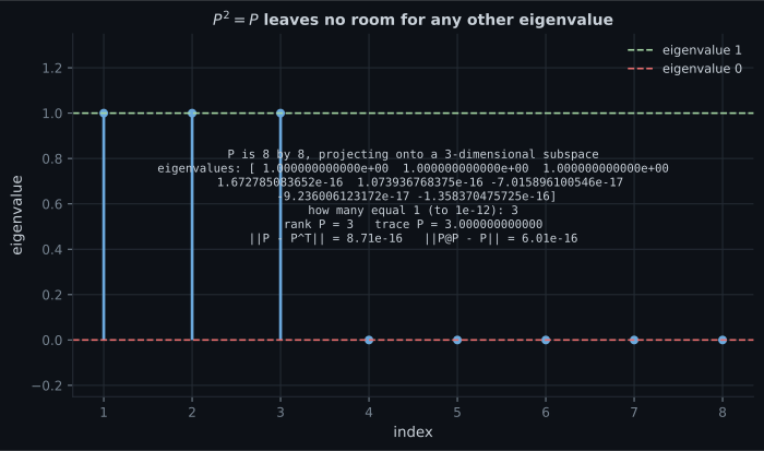
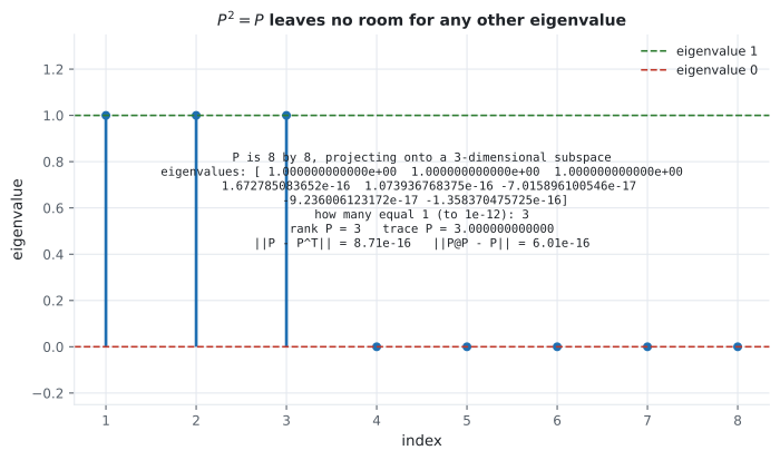
That last pattern is not a coincidence, and it is the cleanest way to recognise a projection matrix: $\mathbf{P}^2 = \mathbf{P}$ forces every eigenvalue to satisfy $\lambda^2 = \lambda$, so $\lambda \in \{0, 1\}$, and the number of ones is the dimension of the subspace. Since the trace is the sum of the eigenvalues, the trace of a projection matrix equals the dimension it projects onto.

Example 3.12 — Gram-Schmidt

$\mathbf{b}_1 = (2,0)^\top$, $\mathbf{b}_2 = (1,1)^\top$.

$\mathbf{u}_1 = \mathbf{b}_1 = (2,0)^\top$, and

$$\mathbf{u}_2 = \mathbf{b}_2 - \frac{\mathbf{u}_1\mathbf{u}_1^\top}{\lVert\mathbf{u}_1\rVert^2}\mathbf{b}_2 = \begin{bmatrix}1\\1\end{bmatrix} - \begin{bmatrix}1&0\\0&0\end{bmatrix}\begin{bmatrix}1\\1\end{bmatrix} = \begin{bmatrix}1\\1\end{bmatrix} - \begin{bmatrix}1\\0\end{bmatrix} = \begin{bmatrix}0\\1\end{bmatrix} \tag{3.71}$$

and $\mathbf{u}_1^\top\mathbf{u}_2 = 0$. The projection matrix $\mathbf{u}_1\mathbf{u}_1^\top/\lVert\mathbf{u}_1\rVert^2 = \mathrm{diag}(1,0)$ is worth a second look: it keeps the first coordinate and discards the second, which is exactly what projecting onto the $x_1$-axis should do.

An affine projection

$L = \mathbf{x}_0 + U$ with $\mathbf{x}_0 = (1,2,-1)^\top$ and $U = \mathrm{span}[(1,1,0)^\top, (0,1,1)^\top]$; project $\mathbf{x} = (4,0,2)^\top$.

step	working	result
shift	$\mathbf{x} - \mathbf{x}_0$	$(3, -2, 3)^\top$
project onto $U$	$\pi_U(3,-2,3)$	$(0.333333,\ 0.666667,\ 0.333333)^\top$
shift back	$\mathbf{x}_0 + \pi_U(\cdot)$	$(1.333333,\ 2.666667,\ -0.666667)^\top$
distance	$\lVert\mathbf{x} - \pi_L(\mathbf{x})\rVert$	$4.618802$
the same, via Eq 3.73b	$d(\mathbf{x}-\mathbf{x}_0,\ \pi_U(\mathbf{x}-\mathbf{x}_0))$	$4.618802$

The two distances agree exactly, which is the content of Equation 3.73: translation does not change distances, so the affine problem never needed its own formula.

book_examples.py

import numpy as np
 
# --- Example 3.10: projection onto a line ---------------------------------
b = np.array([1.0, 2.0, 2.0])
P = np.outer(b, b) / float(b @ b)
print("9 * P =\n", 9 * P)
x = np.array([1.0, 1.0, 1.0])
print("lambda =", float(b @ x) / float(b @ b))
print("9 * pi(x) =", 9 * (P @ x))
print("P^2 = P:", np.allclose(P @ P, P), " rank", np.linalg.matrix_rank(P),
      " trace", round(float(np.trace(P)), 12), " eig", np.round(np.linalg.eigvalsh(P), 12))
 
# --- Example 3.11: projection onto a plane --------------------------------
B = np.array([[1.0, 0.0], [1.0, 1.0], [1.0, 2.0]])
x = np.array([6.0, 0.0, 0.0])
G, c = B.T @ B, B.T @ x
print("B^T B =\n", G, "\nB^T x =", c)
lam = np.linalg.solve(G, c)
pi = B @ lam
err = x - pi
Pm = B @ np.linalg.inv(G) @ B.T
print("lambda =", lam, " pi(x) =", pi)
print("error =", err, " norm =", np.linalg.norm(err), " sqrt(6) =", np.sqrt(6))
print("6 * P =\n", np.round(6 * Pm, 10))
print("B^T error =", np.round(B.T @ err, 12))
print("P^2 = P:", np.allclose(Pm @ Pm, Pm), " rank", np.linalg.matrix_rank(Pm),
      " trace", round(float(np.trace(Pm)), 12), " eig", np.round(np.linalg.eigvalsh(Pm), 12))
 
# --- Affine: shift, project, shift back -----------------------------------
x0 = np.array([1.0, 2.0, -1.0])
Ba = np.stack([np.array([1.0, 1.0, 0.0]), np.array([0.0, 1.0, 1.0])], axis=1)
Q, _ = np.linalg.qr(Ba)
xa = np.array([4.0, 0.0, 2.0])
shifted = xa - x0
pu = Q @ (Q.T @ shifted)
pl = x0 + pu
print("pi_L(x) =", np.round(pl, 6))
print("d(x, L) =", round(float(np.linalg.norm(xa - pl)), 6),
      " via Eq 3.73b =", round(float(np.linalg.norm(shifted - pu)), 6))

output

9 * P =
 [[1. 2. 2.]
 [2. 4. 4.]
 [2. 4. 4.]]
lambda = 0.5555555555555556
9 * pi(x) = [ 5. 10. 10.]
P^2 = P: True  rank 1  trace 1.0  eig [0. 0. 1.]
B^T B =
 [[3. 3.]
 [3. 5.]] 
B^T x = [6. 0.]
lambda = [ 5. -3.]  pi(x) = [ 5.  2. -1.]
error = [ 1. -2.  1.]  norm = 2.449489742783178  sqrt(6) = 2.449489742783178
6 * P =
 [[ 5.  2. -1.]
 [ 2.  2.  2.]
 [-1.  2.  5.]]
B^T error = [0. 0.]
P^2 = P: True  rank 2  trace 2.0  eig [-0.  1.  1.]
pi_L(x) = [ 1.333333  2.666667 -0.666667]
d(x, L) = 4.618802  via Eq 3.73b = 4.618802

Every number in Examples 3.10 and 3.11 reproduces digit for digit, including the $\sqrt{6}$ projection error to sixteen figures and the $\mathbf{B}^\top$ error being exactly zero rather than $10^{-16}$.

See it move

The first sketch is §3.8.1 with everything draggable, and it shows the equality $\lVert\pi_U(\mathbf{x})\rVert = \lvert\cos\omega\rvert\lVert\mathbf{x}\rVert$ live.

sketch Projection onto a line, with the cosine identity live p5.js Pause Restart

Drag x and drag b. The green arrow is the projection, the red dashed segment is the error, and the small square marks the right angle at the foot. The readout gives lambda, both routes to the projection's length, and the check that the error is orthogonal to b — which is the condition the formula was derived from.

The second sketch drops a point cloud onto a line and shows what PCA is choosing between: rotate the line and watch the total squared error and the total projected spread trade off exactly.

sketch Rotate the line: what PCA is actually optimising p5.js Pause Restart

Twenty points, a line through their mean, and every point's projection onto it. Drag the angle knob. The two bars are the total squared projection error and the variance of the projected coordinates, and their sum is constant — so minimising the error and maximising the spread are the same problem, which is the whole of Chapter 10 in one control.

Now the stepped versions of both book examples. First the line, Example 3.10:

vectorExample 3.10, step by stepprojection onto a line, §3.8.1

dim U 1ambient R^3

1lam = (b @ x) / (b @ b)          # the one coordinate2proj = lam * b                   # the closest point on the line3err  = x - proj                  # and what got thrown away4assert abs(b @ err) < tol        # err is orthogonal to b5P = np.outer(b, b) / (b @ b)     # the projection matrix6assert np.allclose(P @ P, P)     # projecting twice changes nothing

setupThe line U is everything of the form λb with b = (1, 2, 2), and x = (1, 1, 1) is not on it. The question is which point of U is closest to x — and "closest" is going to turn out to mean one specific thing.

Play‹›1/7⟲

One direction, so one unknown and no system to solve. The last two frames multiply out the projection matrix and check that squaring it changes nothing.

Then the plane, Example 3.11 — with the normal equation formed and solved on screen:

vectorExample 3.11, step by stepprojection onto a subspace, §3.8.2

dim U 2ambient R^3

1B = np.column_stack(basis)2G = B.T @ B                      # Gram matrix, m by m3c = B.T @ x4lam = np.linalg.solve(G, c)      # the normal equation5proj = B @ lam6err  = x - proj7assert np.allclose(B.T @ err, 0) # orthogonal to every basis vector8P = B @ np.linalg.inv(G) @ B.T   # the pseudo-inverse sandwich9assert np.allclose(P @ P, P)

setupThe subspace U is spanned by (1, 1, 1) and (0, 1, 2), and x = (6, 0, 0) sticks out of it. We want the point of U closest to x, expressed in the basis of U.

Play‹›1/8⟲

Watch the Gram matrix appear, get inverted, and produce lambda = (5, -3). The verification frame measures the inner product of the displacement against each basis vector, and both are exactly zero.

From scratch

projection_from_scratch.py

import numpy as np
 
def project(x, B, ridge=0.0):
    """Project x onto the column span of B, three ways, and check they agree.
 
    `ridge` is the book's jitter term: adding eps*I to B^T B guarantees positive
    definiteness. It changes the answer, which is the point of the pitfall below.
    """
    B = np.atleast_2d(np.asarray(B, dtype=float))
    if B.shape[0] == 1:
        B = B.T
    m = B.shape[1]
 
    # Route 1: the normal equation, as stated in Equation 3.56.
    G = B.T @ B + ridge * np.eye(m)
    lam = np.linalg.solve(G, B.T @ x)
    p1 = B @ lam
 
    # Route 2: the projection matrix of Equation 3.59, formed explicitly.
    P = B @ np.linalg.inv(G) @ B.T
    p2 = P @ x
 
    # Route 3: an orthonormal basis, where everything collapses to B B^T.
    Q, _ = np.linalg.qr(B)
    p3 = Q @ (Q.T @ x)
 
    return {
        "lambda": lam,
        "projection": p1,
        "P": P,
        "error": x - p1,
        "error_norm": float(np.linalg.norm(x - p1)),
        "route_1_vs_2": float(np.linalg.norm(p1 - p2)),
        "route_1_vs_3": float(np.linalg.norm(p1 - p3)),
        "idempotent": float(np.linalg.norm(P @ P - P)),
        "symmetric": float(np.linalg.norm(P - P.T)),
        "orthogonal_residual": float(np.abs(B.T @ (x - p1)).max()),
        "rank": int(np.linalg.matrix_rank(P)),
        "trace": float(np.trace(P)),
    }
 
B = np.array([[1.0, 0.0], [1.0, 1.0], [1.0, 2.0]])
x = np.array([6.0, 0.0, 0.0])
r = project(x, B)
for k in ("lambda", "projection", "error", "error_norm", "route_1_vs_2", "route_1_vs_3",
          "idempotent", "symmetric", "orthogonal_residual", "rank", "trace"):
    v = r[k]
    print(f"{k:22}", np.round(v, 12) if isinstance(v, np.ndarray) else v)
 
# The three routes agree here, but only one of them survives an ill-conditioned
# basis. A polynomial design matrix is the standard way to produce one: the
# monomials 1, t, t^2, ... are very nearly parallel on a short interval.
print()
n = 40
t = np.linspace(0.0, 1.0, n)
rng = np.random.default_rng(5)
y = rng.normal(size=n)
for degree in (5, 7, 9, 11):
    Bd = np.vander(t, degree + 1, increasing=True)
    G = Bd.T @ Bd
    p_normal = Bd @ np.linalg.solve(G, Bd.T @ y)
    Qb, _ = np.linalg.qr(Bd)
    p_qr = Qb @ (Qb.T @ y)
    print(f"degree {degree:3}   cond(B) {np.linalg.cond(Bd):9.2e}   "
          f"cond(B^T B) {np.linalg.cond(G):9.2e}   "
          f"|normal-eq minus QR| {np.linalg.norm(p_normal - p_qr):.3e}")

output

lambda                 [ 5. -3.]
projection             [ 5.  2. -1.]
error                  [ 1. -2.  1.]
error_norm             2.449489742783178
route_1_vs_2           6.280369834735101e-16
route_1_vs_3           6.661338147750939e-16
idempotent             2.6910028968576024e-16
symmetric              0.0
orthogonal_residual    0.0
rank                   2
trace                  1.9999999999999998
 
degree   5   cond(B)  3.48e+03   cond(B^T B)  1.21e+07   |normal-eq minus QR| 7.567e-11
degree   7   cond(B)  1.09e+05   cond(B^T B)  1.18e+10   |normal-eq minus QR| 5.842e-08
degree   9   cond(B)  3.52e+06   cond(B^T B)  1.24e+13   |normal-eq minus QR| 4.811e-06
degree  11   cond(B)  1.18e+08   cond(B^T B)  1.34e+16   |normal-eq minus QR| 4.807e-02

The first block is Example 3.11, verified through three independent routes that agree to $6.7\times10^{-16}$. Note trace printing as $1.9999999999999998$ rather than $2$: the trace of a projection matrix is exactly the dimension mathematically, and two units in the last place numerically.

The second block is the warning, and it is worth reading column by column. cond(B^T B) is the square of cond(B) in every row, so forming the normal equation doubles the digits you lose. The consequence is in the last column: at degree $11$, where $\kappa(\mathbf{B}) = 1.2\times10^{8}$ — not an extreme figure for a polynomial fit — the normal-equation projection is $0.048$ away from the QR answer. That is not a rounding difference, it is a visible error in the fitted values.

A caution about how to demonstrate this, because it is easy to get wrong: if you build a test basis with orthogonal columns and merely shrink them, $\mathbf{B}^\top\mathbf{B}$ comes out diagonal and solving it loses nothing at all, no matter how large the condition number is. The damage comes from nearly-parallel columns, which is why the demonstration above uses a monomial basis rather than a scaled orthogonal one.

On real data

figure A regression fit is a projection matplotlib

The fitted values are P y for the projection matrix onto the column space of the design matrix. X-transpose r comes out at 8e-15 rather than zero only because of floating point: the residual is orthogonal to both columns, which is the normal equation. Rank 2, trace 2.

figure The projection error is the objective PCA minimises matplotlib

Each point is the mean squared error of projecting all 1797 images onto their best k-dimensional subspace. The error reaches exactly zero at k = 61, which is the rank of the centred data, and 21 components suffice for 90% of the variance. The reconstructions underneath are the same projection applied to one image.

figure A projection matrix has only two eigenvalues matplotlib

P squared equals P forces every eigenvalue to satisfy lambda squared equals lambda, so each is 0 or 1. Three of them are exactly 1 — the dimension of the subspace — and the trace is 3.000000000000, which is why the trace of a projection matrix tells you the dimension it projects onto.

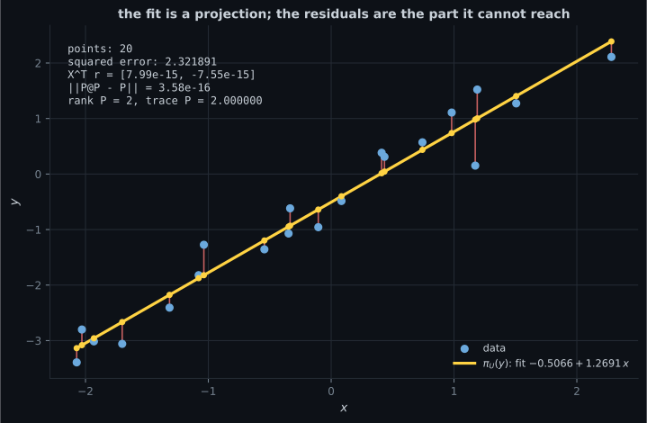
Reading the plot

From the regression figure. The fitted line is $-0.5066 + 1.2691x$ over twenty points, with a squared error of $2.321891$. But the number to read is $\mathbf{X}^\top\mathbf{r} = (8.0\times10^{-15},\ -7.6\times10^{-15})$.

That is the normal equation, measured. Fitting a line by least squares and projecting $\mathbf{y}$ onto the column space of $\mathbf{X}$ are not analogous operations, they are the same operation: the condition that determines the fit is that the residual be orthogonal to every column of the design matrix, which is Equation 3.56 with $\mathbf{B}$ renamed $\mathbf{X}$.

The projection matrix is rank $2$ with trace $2$ — one for the intercept column and one for the slope column — and $\lVert\mathbf{P}^2 - \mathbf{P}\rVert = 3.6\times10^{-16}$. In regression this matrix has its own name, the hat matrix, and its diagonal entries are the leverages. Same object, different vocabulary.

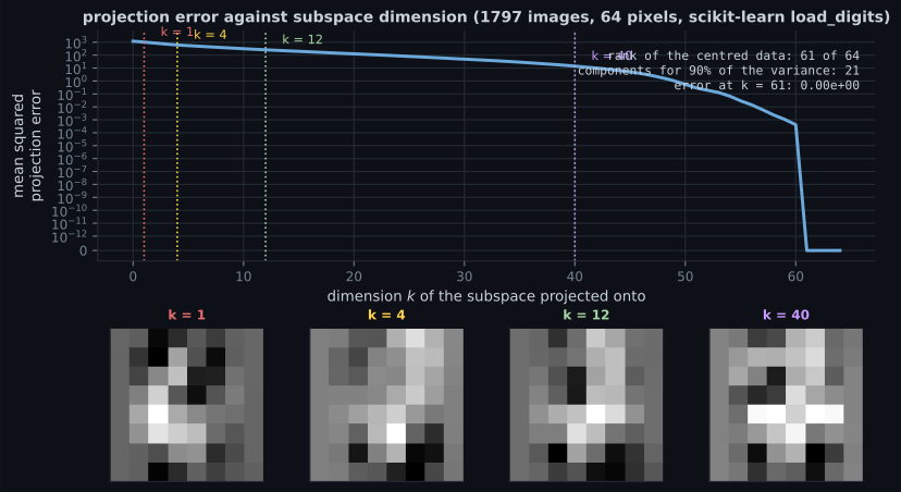
From the digits curve. Four measurements worth having:

$k$	mean squared error	variance kept
1	$1022.5714$	$14.89\%$
4	$616.1911$	$48.71\%$
12	$258.7058$	$78.47\%$
40	$14.1742$	$98.82\%$
61	$0.0000$	$100\%$

The error hits exactly zero at $k = 61$, not at $k = 64$, because the centred data has rank $61$ — which the Orthogonal Complement page traced to three pixels that are zero in all $1797$ images. Beyond $k = 61$ there is nothing left to capture, so the curve does not merely flatten; it terminates.

And $21$ components carry $90\%$ of the variance. Sixty-four numbers per image compressed to twenty-one, at a tenth of the squared error — which is a claim about a projection, computed with Equation 3.59 and nothing else. Chapter 10 will spend a chapter on which subspace is best; the fact that projecting onto a subspace is what you are doing is settled here.

From the spectrum. $\mathbf{P}^2 = \mathbf{P}$ implies $\lambda^2 = \lambda$ for every eigenvalue, so $\lambda \in \{0,1\}$ — measured, three exact ones and five exact zeros. Three consequences follow for free:

• $\mathrm{rank}(\mathbf{P}) = \dim U$, since the rank is the number of nonzero eigenvalues.
• $\mathrm{trace}(\mathbf{P}) = \dim U$, since the trace is their sum. Measured: $3.000000000000$.
• $\mathbf{P}$ is not invertible unless $U$ is the whole space. It throws information away, which is what a projection is for.

That third point is the one people trip over. $\mathbf{P}$ has an inverse only when $\dim U = n$, in which case $\mathbf{P} = \mathbf{I}$ and the projection was doing nothing.

Pitfalls

Never form B-transpose B if you can avoid it

$\kappa(\mathbf{B}^\top\mathbf{B}) = \kappa(\mathbf{B})^2$, so the normal equation loses twice as many digits as the problem requires. The measurement is above: on a degree-11 monomial design with $\kappa(\mathbf{B}) = 1.2\times10^{8}$, the normal-equation projection differs from the QR projection by $0.048$. Use np.linalg.lstsq, or a QR factorisation, both of which work on $\mathbf{B}$ directly. Forming $\mathbf{B}^\top\mathbf{B}$ is fine for a derivation and bad for a computation.

A spanning set is not a basis, and Equation 3.59 requires a basis

The book flags this in a margin note. If $\mathbf{B}$‘s columns are linearly dependent then $\mathbf{B}^\top\mathbf{B}$ is singular and $(\mathbf{B}^\top\mathbf{B})^{-1}$ does not exist. The book’s Exercise 3.5 gives four spanning vectors in $\mathbb{R}^5$ whose rank is only $3$ — Equation 3.59 fails on them as written, while lstsq returns the correct projection regardless, because it uses a minimum-norm pseudo-inverse rather than an inverse.

The jitter term changes the answer

Adding $\varepsilon\mathbf{I}$ to $\mathbf{B}^\top\mathbf{B}$ makes the solve stable and makes the result not a projection: $\mathbf{P}_\varepsilon^2 \neq \mathbf{P}_\varepsilon$, and the “projection” lands strictly inside $U$‘s reach rather than on the closest point. That shrinkage is exactly what ridge regression is for and it is a deliberate bias, not a numerical detail. If you add jitter, you are no longer computing an orthogonal projection; report the $\varepsilon$.

Idempotent does not mean orthogonal

Definition 3.10 asks only for $\pi^2 = \pi$. The matrix $\begin{bmatrix}1 & 1\\ 0 & 0\end{bmatrix}$ satisfies it and is an oblique projection onto the $x_1$-axis: its displacement is not perpendicular to the axis, so its output is not the closest point. Orthogonal projections are exactly the idempotent matrices that are also symmetric — which is why the from-scratch code checks both.

Two different shapes: P is n by n and lambda is m-dimensional

The projection $\pi_U(\mathbf{x})$ still has $n$ ambient coordinates even though it lies in an $m$-dimensional subspace. The compressed representation is $\boldsymbol{\lambda}$, with $m$ numbers. The book makes this a Remark, and it is the difference between “PCA reduces my data to 21 dimensions” (the $\boldsymbol{\lambda}$) and “PCA reconstructs my 64-pixel image” (the $\mathbf{B}\boldsymbol{\lambda}$). Storing the latter saves nothing.

Distances under a non-standard inner product need the matrix in every step

Everything on this page assumed the dot product. Under $\langle\mathbf{x},\mathbf{y}\rangle = \mathbf{x}^\top\mathbf{A}\mathbf{y}$, the normal equation becomes $\mathbf{B}^\top\mathbf{A}\mathbf{B}\boldsymbol{\lambda} = \mathbf{B}^\top\mathbf{A}\mathbf{x}$, and the projection matrix is $\mathbf{B}(\mathbf{B}^\top\mathbf{A}\mathbf{B})^{-1}\mathbf{B}^\top\mathbf{A}$ — which is idempotent but not symmetric. The book’s Remark that one must pay attention to angles and distances under general inner products is doing real work here.

Compare

situation	formula	cost	when to use
line, $\dim U = 1$	$\dfrac{\mathbf{b}\mathbf{b}^\top}{\mathbf{b}^\top\mathbf{b}}\mathbf{x}$	$O(n)$	one direction; always safe
general basis $\mathbf{B}$	$\mathbf{B}(\mathbf{B}^\top\mathbf{B})^{-1}\mathbf{B}^\top\mathbf{x}$	$O(nm^2 + m^3)$	derivations; small well-conditioned $m$
orthonormal basis $\mathbf{Q}$	$\mathbf{Q}\mathbf{Q}^\top\mathbf{x}$	$O(nm)$	whenever you can get one — no solve, no conditioning
in practice	np.linalg.lstsq(B, x)	$O(nm^2)$	numerically the right default; tolerates rank deficiency
affine $L = \mathbf{x}_0 + U$	$\mathbf{x}_0 + \pi_U(\mathbf{x}-\mathbf{x}_0)$	as above	offsets, hyperplanes, bias terms
with a ridge	$\mathbf{B}(\mathbf{B}^\top\mathbf{B}+\varepsilon\mathbf{I})^{-1}\mathbf{B}^\top\mathbf{x}$	as general	deliberate shrinkage; not a projection

pch.quizTag Check your understanding

1. What single condition determines the projection, and where does it come from?

   A That the projection has the same length as x B That the displacement x minus pi(x) is orthogonal to every basis vector of U — because sliding along U from the foot of a perpendicular adds a squared term by Pythagoras, so it can only increase the distance C That the projection matrix is invertible D That the basis is orthonormal
   pch.quizShowAnswer

   B — That the displacement x minus pi(x) is orthogonal to every basis vector of U — because sliding along U from the foot of a perpendicular adds a squared term by Pythagoras, so it can only increase the distance — Stacking that condition over the m basis vectors gives B-transpose (x minus B lambda) equals zero, which is the normal equation. Everything else on the page is bookkeeping on that one line.

2. A projection matrix has trace 3. What do you know?

   A Its largest eigenvalue is 3 B It projects onto a 3-dimensional subspace, because P squared equals P forces every eigenvalue to be 0 or 1 and the trace is their sum C It is 3 by 3 D Nothing without more information
   pch.quizShowAnswer

   B — It projects onto a 3-dimensional subspace, because P squared equals P forces every eigenvalue to be 0 or 1 and the trace is their sum — The measured example on this page is 8 by 8 with trace 3.000000000000, projecting onto a 3-dimensional subspace. The rank equals the trace for the same reason.

3. Why does the from-scratch code warn against forming B-transpose B?

   A It is slower B Its condition number is the square of B's, so the normal equation loses twice as many digits — measured, on a degree-11 monomial design with cond(B) = 1.2e8 the normal-equation projection differs from the QR one by 0.048 C It is not symmetric D It may not be square
   pch.quizShowAnswer

   B — Its condition number is the square of B's, so the normal equation loses twice as many digits — measured, on a degree-11 monomial design with cond(B) = 1.2e8 the normal-equation projection differs from the QR one by 0.048 — It is also the reason classical Gram-Schmidt and the augmented-matrix route to an ONB lose accuracy. The fix is the same in all three cases: work on B directly with a QR factorisation.

4. The digits projection error reaches exactly zero at k = 61 rather than k = 64. Why?

   A Numerical tolerance in the SVD B The centred data has rank 61 — three pixels are zero in all 1797 images — so beyond dimension 61 there is nothing left for a larger subspace to capture C Because 21 components already give 90% of the variance D Because the images are 8 by 8
   pch.quizShowAnswer

   B — The centred data has rank 61 — three pixels are zero in all 1797 images — so beyond dimension 61 there is nothing left for a larger subspace to capture — The Orthogonal Complement page identifies those three pixels as 0, 32 and 39, and shows that they span the orthogonal complement of the data exactly. 61 + 3 = 64.

5. Which matrix is a projection but NOT an orthogonal projection?

   A The identity B [[1, 1], [0, 0]] — it is idempotent, so it is a projection by Definition 3.10, but it is not symmetric, so its displacement is not perpendicular to the target subspace and its output is not the closest point C Any symmetric matrix D B(B-transpose B)-inverse B-transpose
   pch.quizShowAnswer

   B — [[1, 1], [0, 0]] — it is idempotent, so it is a projection by Definition 3.10, but it is not symmetric, so its displacement is not perpendicular to the target subspace and its output is not the closest point — Orthogonal projections are exactly the matrices that are both idempotent and symmetric. Definition 3.10 asks only for idempotence, which is why oblique projections exist and why the from-scratch code checks symmetry separately.

🧪 Try It Yourself

Exercise 1 – Example 3.10 from scratch

pch.exerciseTag pch.exerciseTitle

Exercise 2 – Example 3.11, all five steps

pch.exerciseTag pch.exerciseTitle

Exercise 3 – A projection matrix has only two eigenvalues

pch.exerciseTag pch.exerciseTitle

Exercise 4 – The normal equation loses twice the digits

pch.exerciseTag pch.exerciseTitle

Exercise 5 – The book’s Exercise 3.5: spanning set, not a basis

pch.exerciseTag pch.exerciseTitle

Recall card

• A projection is any linear map with pi squared equal to pi — Definition 3.10. Idempotence alone permits oblique projections; orthogonal projections are the idempotent maps that are also symmetric.
• The condition that determines the answer is that the displacement be orthogonal to every basis vector of the subspace, which is Pythagoras: sliding along the subspace from the foot of a perpendicular only adds a squared term.
• On a line: lambda is b-transpose x over b-transpose b, and the projection matrix is the outer product b b-transpose divided by b-transpose b. It is symmetric and has rank one.
• In general: the normal equation B-transpose B lambda equals B-transpose x, so lambda is the pseudo-inverse applied to x and the projection matrix is B times the inverse Gram matrix times B-transpose.
• With an orthonormal basis everything collapses to lambda equals Q-transpose x and the projector equals Q Q-transpose — no solve and no conditioning problem.
• A projection matrix has eigenvalues zero and one only, so its rank and its trace both equal the dimension of the subspace, and it is never invertible unless it is the identity.
• Gram-Schmidt is this projection used constructively, and the affine case is shift, project, shift back — with the distance unchanged by the shift.
• Least squares is a projection: the residual is orthogonal to every column of the design matrix, measured at eight times ten to the minus fifteen. The projection matrix is the hat matrix.
• PCA minimises the projection error of Equation 3.63. On the digit data the error reaches exactly zero at dimension 61, the rank of the centred data, and twenty-one components carry ninety percent of the variance.
• Never form B-transpose B in production code: its condition number is the square of B’s, and on a degree-11 polynomial design the measured gap between the normal equation and QR reaches 0.048.

Next: Rotations — the transformations that move data without distorting any of the geometry this chapter built.