Maximum Likelihood and Its Obstacle

Chapters 9 and 10 both ended in a formula. This one does not, and the book says so before it starts:

Our “normal” procedure would be to compute the gradient $\mathrm{d}L/\mathrm{d}\boldsymbol\theta$ of the log-likelihood with respect to the model parameters $\boldsymbol\theta$ , set it to $\mathbf{0}$ , and solve for $\boldsymbol\theta$ . However […] we cannot obtain a closed-form solution.

This page is about exactly what that sentence costs, measured on the book’s own seven data points.

What you’ll learn

The book’s running example, reproduced: $\mathcal{X} = \{-3, -2.5, -1, 0, 2, 4, 5\}$ with $K = 3$ initialised at $\mathcal{N}(-4,1)$ , $\mathcal{N}(0,0.2)$ , $\mathcal{N}(8,3)$ — negative log-likelihood $28.325536$ , which is the $28.3$ the book prints.
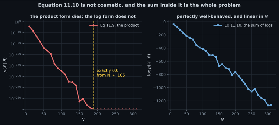
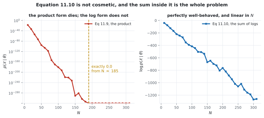
Equations 11.9–11.10, and why the log form is not cosmetic: the product underflows to exactly $0.0$ by about $N = 185$ .
Equation 11.11: with $K = 1$ the log gets inside and there is a closed form — checked against a numerical optimiser to $5.8\times10^{-8}$ .
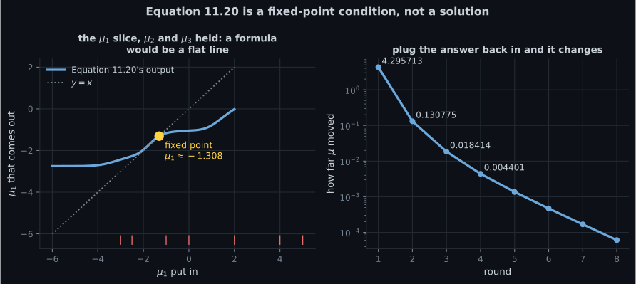
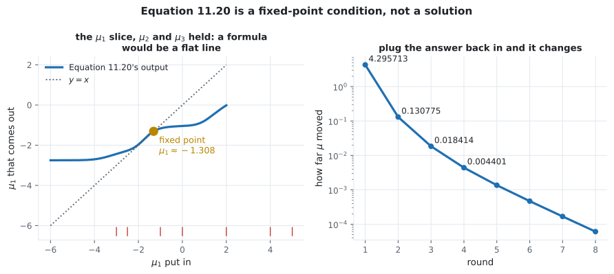
Equations 11.12–11.16, and the precise sense in which Equation 11.20 is not a solution: put $\boldsymbol\mu$ in, get a different $\boldsymbol\mu$ out — measured, by $4.295713$ on the first round.
The analytic gradient of Equation 11.22c, checked against central differences to $3.0\times10^{-10}$ .
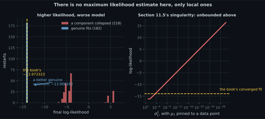
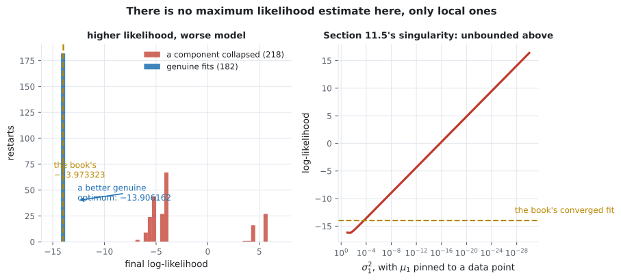
The likelihood surface has many summits. $400$ restarts on seven points find $17$ distinct values — and $218$ of them ( $54.5\%$ ) collapse a component onto a data point.
§11.5’s singularity, measured: pin a mean to a data point and shrink its variance, and the log-likelihood climbs without bound — $+16.377668$ at $\sigma^2 = 10^{-30}$ against the book’s converged $-13.973323$ .
A finding the book does not mention: its own initialisation reaches $-13.973323$ , while a different basin reaches $\mathbf{-13.906162}$ — a genuinely better non-degenerate fit, by $0.067161$ nats.

Intuition: the log cannot get past the sum

Every closed form in Chapters 9 and 10 came from the same accident. The log-likelihood of a Gaussian is a quadratic in the parameters, so setting its derivative to zero gives a linear system, and a linear system you can solve.

Take a mixture and that collapses. Equation 11.10 is $\sum_n \log \sum_k(\cdot)$ , and the outer log cannot be moved inside the inner sum. Differentiate it and every term carries a factor $1/\sum_j \pi_j\mathcal{N}(\cdot)$ — the whole mixture density — so the equation for $\boldsymbol\mu_k$ mentions every other parameter. You get a condition the answer satisfies, not the answer.

diagram Where the closed form goes mermaid

  flowchart TD
  A["log p(X | theta) = sum_n log sum_k pi_k N(...)
Equation 11.10"]
  A -->|"K = 1: the sum vanishes"| B["log N is a quadratic
Equation 11.11"]
  B --> C["set the derivative to 0
-> the sample mean and variance"]
  A -->|"K > 1: the log is stuck outside"| D["every derivative carries 1/p(x_n | theta)
Equations 11.15, 11.16"]
  D --> E["r_nk appears
Equation 11.17"]
  E --> F["mu_k = sum r x / sum r
but r depends on mu"]
  F --> G["iterate: Section 11.3"]

§11.2 The likelihood

For an i.i.d. dataset $\mathcal{X} = \{\mathbf{x}_1,\ldots,\mathbf{x}_N\}$ :

p(\mathcal{X}\mid\boldsymbol\theta) = \prod_{n=1}^{N} p(\mathbf{x}_n\mid\boldsymbol\theta), \qquad p(\mathbf{x}_n\mid\boldsymbol\theta) = \sum_{k=1}^{K}\pi_k\,\mathcal{N}(\mathbf{x}_n\mid\boldsymbol\mu_k,\boldsymbol\Sigma_k) \qquad \text{(11.9)}

\log p(\mathcal{X}\mid\boldsymbol\theta) = \sum_{n=1}^{N}\log\sum_{k=1}^{K}\pi_k\,\mathcal{N}(\mathbf{x}_n\mid\boldsymbol\mu_k,\boldsymbol\Sigma_k) =: L \qquad \text{(11.10)}

On the book’s seven points at its initialisation:

	value
the product, Equation 11.9	$4.993168\times10^{-13}$
its logarithm	$-28.325536$
the sum of logs, Equation 11.10	$-28.325536$ (gap $7.1\times10^{-15}$ )
the negative log-likelihood	$\mathbf{28.325536}$ — the book’s $28.3$

Left, a log-scale curve of the product likelihood falling from about 1e-20 to the bottom of the axis and flat-lining at a dashed vertical marker near N equals 185. Right, the sum of log densities falling smoothly and roughly linearly to about minus 1300. — Both panels show the same likelihood for growing sample sizes. The product form crosses the smallest positive float64 and becomes exactly 0.0 at about N = 185, after which its logarithm is minus infinity. The sum of logs is linear in N and never in trouble.

Numerically, the log turns a product of $N$ small numbers into a sum — measured above, that is the difference between a usable quantity and $0.0$ past $N \approx 185$ .

Analytically, the log usually simplifies the expression. Equation 11.11 is the case where it does:

\log\mathcal{N}(\mathbf{x}\mid\boldsymbol\mu,\boldsymbol\Sigma) = -\tfrac{D}{2}\log(2\pi) - \tfrac12\log\det(\boldsymbol\Sigma) - \tfrac12(\mathbf{x}-\boldsymbol\mu)^\top\boldsymbol\Sigma^{-1}(\mathbf{x}-\boldsymbol\mu)

Measured on the same seven points with $K = 1$ : the closed-form answer is the sample mean $0.6428571429$ and sample variance $8.3367346939$ , and a Nelder–Mead search agrees to $5.8\times10^{-8}$ .

The first benefit survives $K > 1$ . The second does not. That asymmetry is the chapter.

The necessary conditions, and what they are not

Setting the three gradients to zero (Equations 11.12–11.14) requires, by the chain rule,

\frac{\partial\log p(\mathbf{x}_n\mid\boldsymbol\theta)}{\partial\boldsymbol\theta} = \frac{1}{p(\mathbf{x}_n\mid\boldsymbol\theta)}\frac{\partial p(\mathbf{x}_n\mid\boldsymbol\theta)}{\partial\boldsymbol\theta}, \qquad \frac{1}{p(\mathbf{x}_n\mid\boldsymbol\theta)} = \frac{1}{\sum_{j}\pi_j\mathcal{N}(\mathbf{x}_n\mid\boldsymbol\mu_j,\boldsymbol\Sigma_j)} \qquad \text{(11.15), (11.16)}

That denominator is the whole mixture. Every parameter’s equation now mentions every other parameter — which is precisely where the responsibilities of page 1103 come from, and precisely why Equation 11.20 is a fixed-point condition:

Left, an S-shaped blue curve crossing a dotted diagonal line once, with a marked intersection and small tick marks along the bottom showing the seven data points. Right, a log-scale plot of how far the parameter moved each round, falling from about 4.3 to under 1e-4 over eight rounds. — A closed-form solution would be a flat line on the left — output independent of input. Instead the update is a genuine map with a fixed point, and reaching it takes iteration: the first round moves the means by 4.295713, the second by 0.130775, the third by 0.018414.

The gradient itself is exactly what the book derives. Equation 11.22c gives $\partial L/\partial\boldsymbol\mu_k = \sum_n r_{nk}(\mathbf{x}_n-\boldsymbol\mu_k)^\top\boldsymbol\Sigma_k^{-1}$ , and against central differences on the initialisation:

	$k = 1$	$k = 2$	$k = 3$
analytic, Equation 11.22c	$2.671866$	$-4.052278$	$-4.200868$
central differences	$2.671866$	$-4.052278$	$-4.200868$

Largest relative gap: $3.0\times10^{-10}$ . The derivation is right; it just does not solve anything.

The surface, and what is on it

Run the iteration from $400$ random starting points on the same seven numbers:

	count	share
distinct final log-likelihoods	$\mathbf{17}$
runs where a component collapsed ( $\sigma_k^2 < 10^{-6}$ )	$\mathbf{218}$	$54.5\%$
genuine fits	$182$	$45.5\%$
distinct non-degenerate optima	$\mathbf{2}$

Left, a histogram of final log-likelihoods: one tall blue bar at about minus 14 and a scatter of red bars spread from minus 7 up to plus 6. Right, a rising line showing the log-likelihood climbing steadily as the variance axis runs from 1 down to 1e-30, crossing far above a dashed horizontal line. — Every red bar sits to the right of every blue one — the degenerate solutions report a higher likelihood than any genuine fit, up to plus 5.5802 against minus 13.9062. The right panel is why: a component sitting exactly on a data point with a vanishing variance drives the density at that point to infinity, so the likelihood is unbounded above.

Split the $400$ runs by whether any component’s variance collapsed:

	log-likelihood range
the $218$ collapsed runs	$-6.6900$ to $\mathbf{+5.5802}$
the $182$ genuine fits	$-13.9733$ to $-13.9062$

Every degenerate run beats every honest one. And §11.5 names the mechanism: “this happens when the mean of a mixture component is identical to a data point and the covariance tends to $0$ . Then, the likelihood approaches infinity.” Measured by pinning $\mu_1 = -3$ and shrinking:

$\sigma_1^2$	log-likelihood
$10^{-1}$	$-16.174872$
$10^{-4}$	$-13.548611$
$10^{-8}$	$-8.950695$
$10^{-16}$	$+0.259572$
$10^{-30}$	$\mathbf{+16.377668}$

So “the maximum likelihood estimate” does not exist for a GMM with free covariances. Every algorithm in this chapter finds a local optimum, and the useful ones are not the tallest.

Among the $182$ non-degenerate runs there are exactly two distinct optima, and the book’s initialisation does not reach the better one:

	$\log p(\mathcal{X}\mid\boldsymbol\theta)$	$\boldsymbol\mu$	$\boldsymbol\sigma^2$	$\boldsymbol\pi$
from the book’s start	$-13.973323$	$-2.7500,\ -0.5041,\ 3.6446$	$0.0625,\ 0.2506,\ 1.6289$	$0.2857,\ 0.2832,\ 0.4311$
the better basin	$\mathbf{-13.906162}$	$-2.7543,\ 0.2828,\ 4.5051$	$0.0625,\ 1.8561,\ 0.2500$	$0.2737,\ 0.4442,\ 0.2821$

The difference is $0.067161$ nats. Both have well-separated components and a smallest variance of $0.0625$ — neither is degenerate. The second simply puts its narrow third component on $\{4, 5\}$ and lets the middle one cover everything from $-1$ to $2$ .

$51.6\%$ of the non-degenerate runs find the better one, and $23.5\%$ of all $400$ find the book’s. This is §11.4.5’s warning made concrete: “there are no guarantees that EM converges to the maximum likelihood solution.”

pch.quizTag Is the obstacle clear?

Why does Equation 11.10 use a sum of logarithms rather than the product of Equation 11.9?

pch.quizShowAnswer

B — For two reasons: the product underflows to exactly 0.0 by about N = 185, and the log usually simplifies the algebra — The numerical benefit survives any K. The analytic one does not: at K = 1 the log lands directly on the Gaussian and gives a closed form, and at K greater than 1 it is stuck outside a sum. That asymmetry is what the rest of the chapter is about.
In what sense is Equation 11.20 not a solution for the means?

pch.quizShowAnswer

B — Its right-hand side depends on the means through the responsibilities, so feeding the answer back in changes it — measured, by 4.295713 on the first round — The chain rule brings 1 over the whole mixture density into every derivative, so each parameter's equation mentions every other parameter. The result is a fixed-point condition. Plotted against its input it is an S-shaped curve crossing the diagonal, where a formula would be a flat line.
400 random restarts on seven data points produced how many distinct final log-likelihoods?

pch.quizShowAnswer

B — Seventeen, of which 218 runs had collapsed a component onto a data point — 54.5 percent of runs collapsed a component, and those report higher likelihoods than any genuine fit — up to plus 5.5802 against minus 13.9062. Among the 182 honest runs there are exactly two optima, and the book's initialisation reaches the worse one by 0.067161 nats.
What happens to the likelihood if a component's mean sits exactly on a data point and its variance shrinks?

pch.quizShowAnswer

B — It grows without bound — measured at plus 16.377668 for a variance of 1e-30 — Section 11.5 names this. Because the likelihood is unbounded above, the maximum likelihood estimate for a GMM with free covariances does not exist, and every algorithm in the chapter is finding a local optimum. The tallest points on the surface are not models.

Exercises

Exercise 1 – Reproduce the book’s 28.3

Exercise 2 – Watch the product die

Exercise 3 – Where the closed form still exists

Exercise 4 – Put the answer in, get a different answer out

Exercise 5 – Climb the singularity

Recall card

The book’s running example is seven numbers, three components initialised deliberately badly, and a negative log-likelihood of 28.325536 — the 28.3 it prints.
Equation 11.10 takes the log for two reasons, and only one of them survives K greater than one.
Numerically: the product of Equation 11.9 underflows to exactly zero by about two hundred data points, and its logarithm becomes minus infinity.
Analytically: at K equal to one the log lands directly on the Gaussian, Equation 11.11, and the answer is the sample mean and sample variance — confirmed by an optimiser to 6e-08.
At K greater than one the log is stuck outside a sum, so the chain rule drags one over the whole mixture density into every derivative.
Which means every parameter’s equation mentions every other parameter. Equation 11.20 is a condition the answer satisfies, not the answer.
Measured, feeding the means back in moves them by 4.295713 on the first round, then 0.130775, then 0.018414. A formula would move them by zero.
The analytic gradient is right — it matches central differences to 3e-10 — it simply cannot be solved.
Four hundred restarts on seven points find seventeen distinct optima.
Two hundred and eighteen of them, 54.5 percent, collapse a component onto a data point, and every one of those reports a higher likelihood than every genuine fit.
The likelihood is unbounded above: pin a mean to a data point and shrink its variance and the log-likelihood reaches plus 16.377668 at 1e-30. So the maximum likelihood estimate does not exist.
Among the honest fits there are exactly two optima, and the book’s own initialisation reaches the worse one — minus 13.973323 against an available minus 13.906162.

Next: Responsibilities — §11.2.1, the quantity that appeared in every derivative above, and what it means.

pch.coffeeTagline

pch.coffeeCta

pch.feedbackHeading

pch.feedbackSubheading