
K-Means Clustering Algorithm
What you’ll learn
Section titled “What you’ll learn”- the k-means objective, and why the two update steps fall out of it
- a proof that Lloyd’s algorithm terminates, and why that does not mean it finds the best answer
- a full iteration worked by hand on six points
- why
n_initexists, measured: inertia 302.46 versus 971.25 from one unlucky start - the elbow and the silhouette, and which one actually answers “how many clusters?”
- three geometries where k-means fails, with adjusted Rand indices attached
- k-means++ , MiniBatchKMeans, and when each pays off
Intuition
Section titled “Intuition”k-means answers one question: if you had to replace every point with one of representative points, which would lose the least information?
Those representatives are the centroids. Once you have them, every point belongs to whichever is nearest. Once you have the assignment, the best possible representative for a group is its mean. Neither half can be solved without the other, so the algorithm alternates: fix the centroids and reassign, fix the assignment and recompute the centroids. Repeat until nothing moves.
That is the entire algorithm. Everything else on this page is consequences of it.
  flowchart TD
  A["Pick k initial centroids
(k-means++ by default)"] --> B["ASSIGN
each point to its nearest centroid"]
  B --> C["UPDATE
each centroid to the mean of its points"]
  C --> D{"Did any assignment change?"}
  D -->|"yes"| B
  D -->|"no"| E["Converged.
Record inertia."]
  E --> F{"Ran n_init times?"}
  F -->|"no"| A
  F -->|"yes"| G["Keep the run with the lowest inertia"]
The math
Section titled “The math”Let partition the points and let be the centroid of . k-means minimises the within-cluster sum of squares, which scikit-learn calls inertia:
Both update rules are the exact minimisers of with the other variable held fixed.
The assignment step. With the centroids fixed, is a sum of independent per-point terms. Each is minimised by choosing the nearest centroid:
The update step. With the assignment fixed, differentiate the contribution of one cluster with respect to its centroid:
Setting this to zero gives , so
The centroid is the mean. Not an approximation — the exact minimiser. This is also why k-means is tied to squared Euclidean distance: swap in and the optimal representative becomes the median, which is a different algorithm (k-medians).
Why it always stops
Section titled “Why it always stops”Both steps are guaranteed not to increase :
- The assignment step moves points only to a centroid that is nearer or equally near, so every term in the sum weakly decreases.
- The update step replaces each centroid with the exact minimiser for its cluster, so each cluster’s contribution weakly decreases.
So is non-increasing. There are only finitely many ways to partition points into groups, and is determined by the partition. A non-increasing sequence over a finite set of values that never revisits a partition must halt. Lloyd’s algorithm always terminates, typically in a handful of iterations.
It terminates at a local minimum. There is no guarantee it is the global one, and finding the
global optimum of is NP-hard even for . That gap is what n_init exists to paper over.
Worked example by hand
Section titled “Worked example by hand”Six one-dimensional points: . Take and the deliberately awkward initial centroids , .
Iteration 1 — assign. Compare against :
| to | to | goes to | |
|---|---|---|---|
| 1 | 1 | 3 | |
| 2 | 0 | 2 | |
| 3 | 1 | 1 | (tie, lowest index) |
| 10 | 8 | 6 | |
| 11 | 9 | 7 | |
| 12 | 10 | 8 |
Iteration 1 — update.
Iteration 2 — assign. With centroids at 2 and 11, points are all nearer 2 (distances 1, 0, 1 against 10, 9, 8) and are all nearer 11. No assignment changed, so the algorithm stops.
Final inertia:
Now watch what a bad start does. Initialise at , instead:
- Assign: ; everything else is nearer 2, so .
- Update: , .
- Assign: is 3 nearer 1 or 7.6? against — nearer 1. So and .
- Update: back to , . Same answer, one iteration later.
This particular bad start recovers. Many do not, which is the next section.
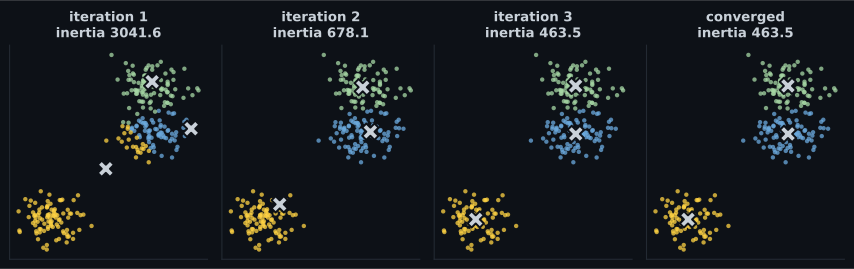
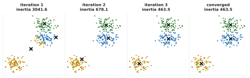
See it move
Section titled “See it move”Initialisation is not a detail
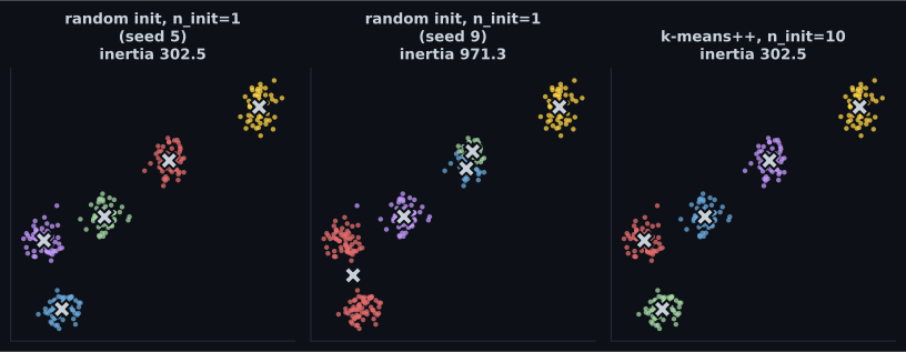
Section titled “Initialisation is not a detail”Run k-means on five well-separated blobs with a single random start and you get a different answer depending on nothing but the seed:
| Initialisation | Inertia |
|---|---|
init="random", n_init=1, seed 5 | 302.46 |
init="random", n_init=1, seed 9 | 971.25 |
init="k-means++", n_init=10 | 302.46 |
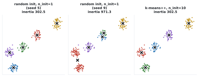
The seed-9 run is over three times worse. Look at what happened: two centroids landed inside the same blob and split it, leaving two genuine blobs merged into one cluster. Both steps of the algorithm behave perfectly; there is simply no single-point reassignment that escapes.
k-means++
Section titled “k-means++”Rather than sampling initial centroids uniformly, k-means++ spreads them out:
- Choose the first centroid uniformly at random from the data.
- For each remaining point , compute , the distance to the nearest centroid already chosen.
- Choose the next centroid from the data with probability proportional to .
- Repeat until centroids are chosen.
The squared weighting makes far-away points overwhelmingly likely to be picked, so the seeds tend to land one per blob. The theoretical guarantee is that the expected inertia is within of the global optimum — before a single Lloyd iteration runs.
This is scikit-learn’s default, and n_init defaults to "auto" (1 for k-means++, 10 for
"random"). If you are doing anything that matters, set n_init=10 explicitly.
Choosing k
Section titled “Choosing k”Inertia cannot choose for you. It falls monotonically — with every point is its own centroid and . Here is that fall, on 400 points containing 4 genuine blobs:
| Inertia | Silhouette | |
|---|---|---|
| 1 | 16534.68 | — |
| 2 | 6850.11 | 0.5723 |
| 3 | 1842.91 | 0.7329 |
| 4 | 646.92 | 0.7475 |
| 5 | 584.31 | 0.6277 |
| 6 | 526.73 | 0.5359 |
| 7 | 474.91 | 0.4494 |
| 8 | 424.39 | 0.3214 |
| 9 | 373.48 | 0.3394 |
| 10 | 341.73 | 0.3511 |
The elbow method looks for the kink where the marginal improvement collapses. From to inertia drops by 1196; from 4 to 5 it drops by 63. That is the elbow, and it points at 4.
The silhouette has an actual maximum at 0.7475, also at . When the two agree, you are done. When they disagree, trust the silhouette — the elbow is a judgement call about the shape of a curve, while the silhouette is a number you can argmax.
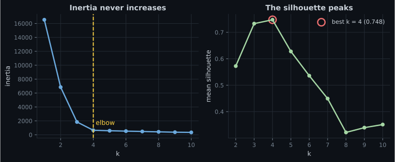
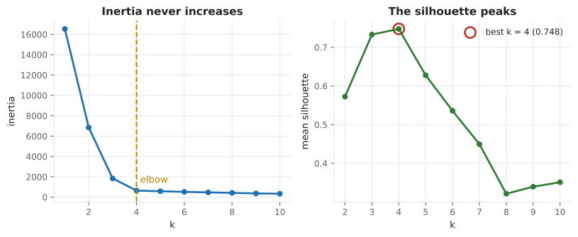
Neither is authoritative. On real data the curve is often smooth with no elbow at all, and the silhouette peaks at because two coarse groups always look cleanly separated. When that happens, the domain decides: how many customer segments can your marketing team actually operate?
Straight-edged cells
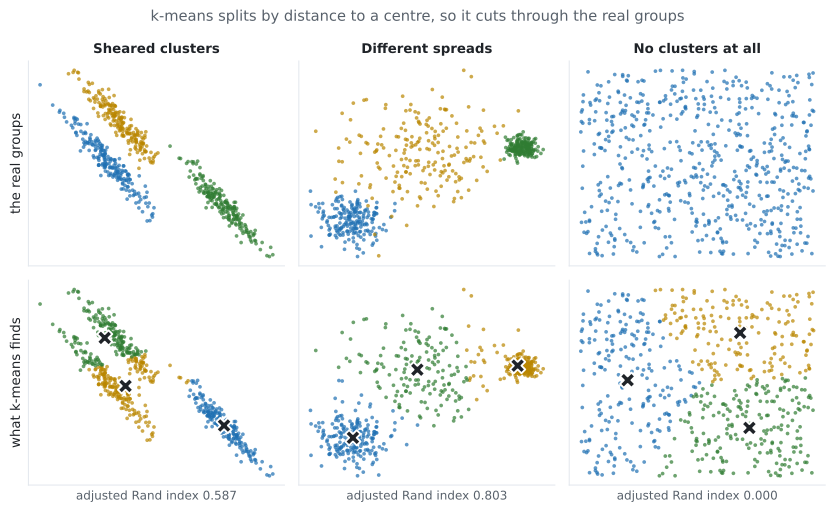
Section titled “Straight-edged cells”Because assignment compares squared distances to centroids, the boundary between two clusters is the set of points equidistant from both — a straight line, and in higher dimensions a hyperplane: the perpendicular bisector of the segment joining them. The partition of space is a Voronoi diagram.
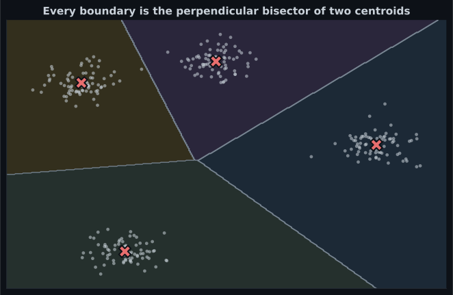
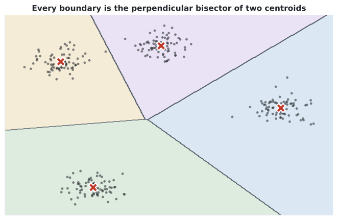
This single geometric fact explains every k-means failure in the next section.
Where it fails
Section titled “Where it fails”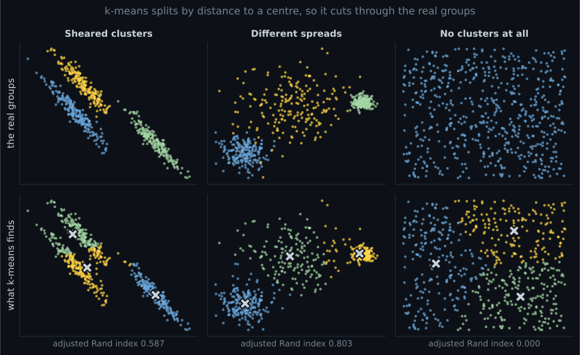
| Failure | Why | What to use instead |
|---|---|---|
| Sheared / elongated clusters | Voronoi cells are isotropic; a stretched cluster costs less to cut across than along | Gaussian mixture with covariance_type="full" |
| Very different spreads | Squared distance charges the wide cluster more, so it loses points to tight neighbours | Gaussian mixture, or DBSCAN if densities differ enough |
| Non-convex shapes (moons, rings) | Straight boundaries cannot bend | DBSCAN, spectral clustering |
| No structure at all | Nothing in the algorithm can say “there are no clusters” | Compare the silhouette against a shuffled null |
| Outliers | The mean is not robust; one distant point drags a centroid | k-medoids, or remove outliers first |
The uniform-noise case deserves emphasis. Silhouette 0.378 is not obviously bad — you would plausibly ship that. The defence is to compare against a null: shuffle each column independently (destroying the joint structure but preserving the marginals), cluster the shuffled data, and check that your real silhouette is meaningfully higher.
In code
Section titled “In code”import numpy as np
from sklearn.cluster import KMeans
from sklearn.datasets import make_blobs
X, _ = make_blobs(n_samples=280, centers=3, cluster_std=0.95, random_state=4)
km = KMeans(n_clusters=3, n_init=10, random_state=0).fit(X)
print("inertia ", round(km.inertia_, 4))
print("iterations", km.n_iter_)
print("centroids\n", km.cluster_centers_.round(3))
print("labels (first 10)", km.labels_[:10])
# The only clustering estimator in this phase that can label unseen points.
print("new point ->", km.predict([[0.0, 0.0]]))
# transform() returns distance to every centroid — often more useful than the label
print("distances ->", km.transform([[0.0, 0.0]]).round(3))from sklearn.cluster import KMeans
from sklearn.datasets import make_blobs
from sklearn.metrics import silhouette_score
X, _ = make_blobs(n_samples=400, centers=4, cluster_std=0.9, random_state=11)
for k in range(1, 11):
km = KMeans(n_clusters=k, n_init=10, random_state=0).fit(X)
sil = silhouette_score(X, km.labels_) if k > 1 else float("nan")
print(f"k={k:2d} inertia {km.inertia_:9.2f} silhouette {sil:.4f}")
# k= 1 inertia 16534.68 silhouette nan
# k= 2 inertia 6850.11 silhouette 0.5723
# k= 3 inertia 1842.91 silhouette 0.7329
# k= 4 inertia 646.92 silhouette 0.7475 <- both agree
# k= 5 inertia 584.31 silhouette 0.6277MiniBatchKMeans
Section titled “MiniBatchKMeans”Full k-means touches every point on every iteration. MiniBatchKMeans samples a small batch each
step and nudges the affected centroids toward it, which turns the per-iteration cost from
into for batch size .
The price is a slightly worse optimum. On 100,000 points in 8 blobs, MiniBatch’s inertia came out 0.04% higher than full k-means; at 500,000 points, 0.01% higher. That is nothing. Use it whenever is large enough that full k-means is inconvenient.
from sklearn.cluster import KMeans, MiniBatchKMeans
from sklearn.datasets import make_blobs

X, _ = make_blobs(n_samples=100_000, centers=8, cluster_std=1.0, random_state=0)

full = KMeans(n_clusters=8, n_init=3, random_state=0).fit(X)
mini = MiniBatchKMeans(n_clusters=8, n_init=3, batch_size=1024, random_state=0).fit(X)

print("full     ", round(full.inertia_, 1))            # 179598.7
print("minibatch", round(mini.inertia_, 1))            # 179671.3
print(f"penalty   {100 * (mini.inertia_ / full.inertia_ - 1):.2f}%")   # 0.04%
Wall-clock timings vary far too much with thread count and BLAS build to quote a speedup you can
rely on. The algorithmic claim is the durable one: each MiniBatch iteration reads batch_size
rows instead of all .
pch.algoApi sklearn.cluster.KMeans
pch.algoAssumes
- Clusters are convex and roughly spherical
- Clusters have comparable spread
- Clusters have comparable numbers of points
- Squared Euclidean distance is the right notion of similarity
- You know k, or can defend a choice of it
pch.algoCost
- pch.algoTrain
O(n k p i) per run, times n_init runs- pch.algoPredict
O(k p) per point- pch.algoMemory
O(n p + k p)
J — inertia (within-cluster sum of squares); mu_j — centroid of cluster j; C_j — the points assigned to j
pch.algoHyperparams
-
n_clustersdefault 8 The whole answer. Choose with the silhouette, the elbow, or the domain. -
initdefault 'k-means++' Spreads the seeds out. Expected inertia within O(log k) of optimal before iterating. -
n_initdefault 'auto' (1 for k-means++) Restarts. Set to 10 for anything that matters: 302.46 vs 971.25 on this page's data. -
max_iterdefault 300 Rarely binds — convergence usually takes under 20 iterations. -
toldefault 1e-4 Stops when the centroid shift falls below this. Loosen for speed on huge data. -
algorithmdefault 'lloyd' 'elkan' uses the triangle inequality to skip distance computations; faster on well-separated data.
pch.algoReachFor
- Clusters are blob-shaped and you roughly know how many
- You need to label new points later (k-means can; DBSCAN cannot)
- n is large — this is the most scalable clustering algorithm in the phase
- You want centroids as an interpretable summary of each group
pch.algoLookElsewhere
- Clusters are elongated, nested, or ring-shaped
- Cluster sizes or densities differ a lot
- The data has outliers you have not handled
- You cannot justify any particular k
Pitfalls
Section titled “Pitfalls”Leaving n_init at the default. Measured above: 971.25 against 302.46, on well-separated
blobs. On messier data the gap is worse. n_init=10 costs ten times the compute of a sub-second
fit.
Arg-minimising inertia over k. Inertia is monotonically decreasing in ; the argmin is always . Use it for the elbow’s shape, never for its minimum.
Not scaling. Covered on the
previous page:
one StandardScaler moved ARI from 0.035 to 0.891.
Trusting cluster indices across runs. Cluster 0 changes identity with random_state. If you
persist labels, persist the centroids and re-derive.
Applying k-means to one-hot encoded categoricals. The mean of a set of one-hot vectors is a vector of proportions, which is not a valid category. Use k-modes, or embed first.
Believing the clusters are real. k-means returns exactly groups from uniform noise, with a silhouette of 0.378. Always compare against a shuffled null.
Forgetting outliers move centroids. One point at distance 100 contributes 10,000 to the objective and will visibly drag its centroid. Handle outliers before clustering, or run a robust detector first.
Compare
Section titled “Compare”| k-means | k-medoids | Gaussian mixture | MiniBatchKMeans | |
|---|---|---|---|---|
| Representative | mean | an actual data point | mean + covariance | mean |
| Distance | squared Euclidean | any metric | Mahalanobis | squared Euclidean |
| Cluster shape | spherical | metric-dependent | ellipsoidal | spherical |
| Robust to outliers | no | yes | no | no |
| Soft assignment | no | no | yes | no |
| Cost per iteration | ||||
| Scales to millions | yes | no | moderate | yes |
-
Why is the centroid update step the MEAN of the assigned points, rather than the median?
Differentiating the sum of squared distances with respect to the centroid and setting the derivative to zero gives exactly the mean. If the objective used absolute distances instead, the minimiser would be the median — that algorithm is k-medians.
pch.quizShowAnswer
B — Because the objective is a sum of SQUARED distances, and the mean is its exact minimiser — Differentiating the sum of squared distances with respect to the centroid and setting the derivative to zero gives exactly the mean. If the objective used absolute distances instead, the minimiser would be the median — that algorithm is k-medians.
-
Lloyd's algorithm is guaranteed to terminate. What is it NOT guaranteed to do?
Both steps weakly decrease inertia and there are finitely many partitions, so it halts. But it halts at a local minimum — finding the global one is NP-hard even for k=2. That is what n_init is for.
pch.quizShowAnswer
B — Find the global minimum of the inertia — Both steps weakly decrease inertia and there are finitely many partitions, so it halts. But it halts at a local minimum — finding the global one is NP-hard even for k=2. That is what n_init is for.
-
You plot inertia against k and it falls smoothly with no visible elbow. What now?
Inertia's minimum is always k=n, so its argmin is useless. The silhouette has a genuine maximum, and when even that is flat the honest answer is that the data has no strong k — pick the number your downstream process can actually use.
pch.quizShowAnswer
B — Check the silhouette, and if that is also flat let the domain decide — Inertia's minimum is always k=n, so its argmin is useless. The silhouette has a genuine maximum, and when even that is flat the honest answer is that the data has no strong k — pick the number your downstream process can actually use.
-
Why can k-means never produce a crescent-shaped cluster?
The set of points equidistant from two centroids is a hyperplane. The partition is therefore a Voronoi diagram with straight edges, and no amount of iteration bends them. Density-based methods have no such constraint.
pch.quizShowAnswer
B — Because assignment is by distance to a centroid, so every boundary is a straight perpendicular bisector — The set of points equidistant from two centroids is a hyperplane. The partition is therefore a Voronoi diagram with straight edges, and no amount of iteration bends them. Density-based methods have no such constraint.
-
MiniBatchKMeans on 100,000 points gave inertia 0.04% higher than full k-means. What does that tell you?
A 0.04% inertia penalty is far below the run-to-run variation you get from different seeds. Each MiniBatch iteration reads batch_size rows instead of all n, so its cost per iteration does not grow with the dataset.
pch.quizShowAnswer
B — The approximation cost is negligible, so use it whenever n makes full k-means inconvenient — A 0.04% inertia penalty is far below the run-to-run variation you get from different seeds. Each MiniBatch iteration reads batch_size rows instead of all n, so its cost per iteration does not grow with the dataset.
🧪 Try It Yourself
Section titled “🧪 Try It Yourself”Exercise 1 – One iteration by hand, in code
Section titled “Exercise 1 – One iteration by hand, in code”Exercise 2 – Prove the mean minimises the objective
Section titled “Exercise 2 – Prove the mean minimises the objective”Exercise 3 – What one bad seed costs
Section titled “Exercise 3 – What one bad seed costs”Exercise 4 – Confidently clustering pure noise
Section titled “Exercise 4 – Confidently clustering pure noise”Exercise 5 – Sheared clusters break it
Section titled “Exercise 5 – Sheared clusters break it”- k-means minimises the within-cluster sum of squares; assignment and mean-update are the exact minimisers of that objective with the other variable held fixed.
- It always terminates — non-increasing objective, finitely many partitions — but only at a local minimum.
- The worked example converged to centroids 2 and 11 with inertia 4 in two iterations.
- Initialisation matters enormously: 971.25 versus 302.46 from nothing but a different seed.
Set
n_init=10. - Inertia cannot pick (it is monotone in ). The silhouette can: it peaked at 0.7475 for .
- Boundaries are straight perpendicular bisectors, so sheared (ARI 0.587) and unequal-spread (ARI 0.803) geometries break it — and pure noise still yields three confident clusters.
- MiniBatchKMeans costs 0.04% inertia at 100k points and reads a fixed batch per iteration.
Exercise 6 – Measure the seed lottery
Section titled “Exercise 6 – Measure the seed lottery”Hierarchical Clustering (Dendrograms) — a method that does not need up front, builds the whole nesting of clusters at once, and lets you choose the cut afterwards.
pch.coffeeTagline
pch.coffeeCtapch.feedbackHeading
pch.feedbackSubheading