Eigenvalues and Eigenvectors

Most vectors, hit by a matrix, come out both turned and stretched. A few special ones come out only stretched — same direction, different length. Those are the eigenvectors, and the stretch factors are the eigenvalues.

The word is German: eigen means “characteristic”, “self” or “own”. These are the matrix’s own directions, and finding them tells you what the matrix is actually doing, in a way that reading its entries never does.

What you’ll learn

• Definition 4.6, the eigenvalue equation, and the four equivalent conditions for $\lambda$ to be an eigenvalue.
• The characteristic polynomial as the route to the eigenvalues (Theorem 4.8), and why it is not how anyone computes them.
• Algebraic against geometric multiplicity (Definitions 4.9 and 4.11), and what defective means (Definition 4.13).
• The spectral theorem (Theorem 4.15): symmetric matrices always have an orthonormal eigenbasis and real eigenvalues.
• Theorems 4.16 and 4.17: $\det\mathbf{A} = \prod\lambda_i$ and $\mathrm{tr}\,\mathbf{A} = \sum\lambda_i$.
• Why a rotation has no real eigenvectors, and why that is the right answer rather than a failure.
• PageRank as the dominant eigenvector of a transition matrix, with the measured convergence rate.

Intuition: the directions a map does not turn

Take a matrix and feed it every direction on the unit circle. Watch the angle between $\mathbf{x}$ and $\mathbf{A}\mathbf{x}$ as you sweep round.

For most directions that angle is nonzero: the matrix turned the vector. At a few special angles it drops to zero (or to $180°$, which is the same line pointing the other way). Those are the eigenvector directions, and the ratio of lengths there is the eigenvalue.

Three things follow immediately, and each is a theorem later:

• There are at most $n$ of these directions, because you cannot have more than $n$ independent directions in $\mathbb{R}^n$.
• There can be fewer. A shear turns every direction except one. A rotation turns every direction, so it has none at all — over the reals.
• A negative eigenvalue is still an eigenvector: the line is preserved, the arrow flips along it.

diagram Diagram mermaid

  flowchart TD
  EQ["Ax = λx, x ≠ 0
Def 4.6"]
  EQ --> HOM["(A − λI)x = 0 has a nonzero solution"]
  HOM --> SING["so A − λI is singular"]
  SING --> DET["so det(A − λI) = 0"]
  DET --> CP["λ is a root of the
characteristic polynomial
Thm 4.8"]
  CP --> ALG["algebraic multiplicity:
how many times the root repeats
Def 4.9"]
  HOM --> ES["eigenspace E_λ = ker(A − λI)
Def 4.10"]
  ES --> GEO["geometric multiplicity:
dim E_λ
Def 4.11"]
  ALG --> CMP["geom ≤ alg, always"]
  GEO --> CMP
  CMP --> DEF["geom sum < n ⟹ DEFECTIVE
Def 4.13, no eigenbasis"]
  CP --> THM["det A = ∏λᵢ (Thm 4.16)
tr A = Σλᵢ (Thm 4.17)"]
  EQ --> SPEC["A symmetric ⟹ real λ and an
ORTHONORMAL eigenbasis
Thm 4.15, the spectral theorem"]

The math

Definition 4.6 — Eigenvalue and eigenvector

Let $\mathbf{A} \in \mathbb{R}^{n\times n}$. Then $\lambda \in \mathbb{R}$ is an eigenvalue of $\mathbf{A}$ and $\mathbf{x} \in \mathbb{R}^n\setminus\{\mathbf{0}\}$ is the corresponding eigenvector if

$$\mathbf{A}\mathbf{x} = \lambda\mathbf{x} \tag{4.25}$$

This is the eigenvalue equation.

The exclusion $\mathbf{x} \neq \mathbf{0}$ is not pedantry. $\mathbf{A}\mathbf{0} = \lambda\mathbf{0}$ holds for every $\lambda$, so without it every number would be an eigenvalue of every matrix.

Four equivalent statements

$$\lambda \text{ is an eigenvalue of } \mathbf{A} \iff \exists\,\mathbf{x}\neq\mathbf{0}: \mathbf{A}\mathbf{x} = \lambda\mathbf{x} \iff (\mathbf{A}-\lambda\mathbf{I})\mathbf{x} = \mathbf{0} \text{ nontrivially}$$ $$\iff \mathrm{rk}(\mathbf{A}-\lambda\mathbf{I}) < n \iff \det(\mathbf{A}-\lambda\mathbf{I}) = 0$$

Read that chain forwards and it is the derivation of the whole method. An eigenvector is a nonzero solution of a homogeneous system, a homogeneous system has a nonzero solution exactly when its matrix is rank-deficient, and a square matrix is rank-deficient exactly when its determinant vanishes (§4.1, Theorem 4.3). So the eigenvalues are the roots of $\det(\mathbf{A}-\lambda\mathbf{I})$, which §4.1 named the characteristic polynomial.

Theorem 4.8

$\lambda \in \mathbb{R}$ is an eigenvalue of $\mathbf{A} \in \mathbb{R}^{n\times n}$ if and only if it is a root of the characteristic polynomial $p_{\mathbf{A}}(\lambda)$.

Eigenvectors are not unique

Remark after Definition 4.7

If $\mathbf{x}$ is an eigenvector of $\mathbf{A}$ with eigenvalue $\lambda$, then for any $c \in \mathbb{R}\setminus\{0\}$,

$$\mathbf{A}(c\mathbf{x}) = c\mathbf{A}\mathbf{x} = c\lambda\mathbf{x} = \lambda(c\mathbf{x}) \tag{4.26}$$

so $c\mathbf{x}$ is an eigenvector with the same eigenvalue. Every vector collinear with $\mathbf{x}$ is one too.

An eigenvector is really a direction, or more precisely a line through the origin. Definition 4.7 distinguishes codirected (same direction) from collinear (same or opposite direction), and eigenvectors come in collinear families. This is why libraries return unit vectors, and why their signs are arbitrary — a fact that costs people reproducibility bugs in PCA plots.

Eigenspaces and multiplicity

Definitions 4.9, 4.10, 4.11

The algebraic multiplicity of $\lambda_i$ is the number of times it appears as a root of the characteristic polynomial.

The eigenspace $E_\lambda$ is the set of all eigenvectors for $\lambda$, together with $\mathbf{0}$ — it is the null space of $\mathbf{A}-\lambda\mathbf{I}$ (Equations 4.27a and 4.27b), hence a subspace. The set of all eigenvalues is the eigenspectrum, or spectrum.

The geometric multiplicity of $\lambda_i$ is $\dim E_{\lambda_i}$: the number of linearly independent eigenvectors associated with it.

Remark after Definition 4.11

The geometric multiplicity is at least 1 (every eigenvalue has at least one eigenvector) and cannot exceed the algebraic multiplicity — but it may be lower.

That inequality is the entire subtlety of this section, and §4.4 depends on it.

Defective matrices

Theorem 4.12 and Definition 4.13

Theorem 4.12. The eigenvectors $\mathbf{x}_1,\dots,\mathbf{x}_n$ of a matrix with $n$ distinct eigenvalues are linearly independent — so they form a basis of $\mathbb{R}^n$.

Definition 4.13. A square matrix is defective if it possesses fewer than $n$ linearly independent eigenvectors.

Distinct eigenvalues are sufficient for an eigenbasis, not necessary. What is required is that the eigenspace dimensions add to $n$; a defective matrix has some $\lambda_i$ with algebraic multiplicity $m > 1$ and geometric multiplicity below $m$. And the book’s remark closes the loop: a defective matrix cannot have $n$ distinct eigenvalues, since Theorem 4.12 would then give it a basis.

Useful properties

• $\mathbf{A}$ and $\mathbf{A}^\top$ have the same eigenvalues, though generally different eigenvectors.
• $E_\lambda = \ker(\mathbf{A}-\lambda\mathbf{I})$.
• Similar matrices have the same eigenvalues, so the eigenvalues — like the determinant and the trace — characterise the mapping, not the representation.
• Symmetric positive definite matrices always have positive, real eigenvalues.

Symmetrising, and the spectral theorem

Theorem 4.14

For any $\mathbf{A} \in \mathbb{R}^{m\times n}$, the matrix

$$\mathbf{S} := \mathbf{A}^\top\mathbf{A} \in \mathbb{R}^{n\times n} \tag{4.36}$$

is symmetric and positive semidefinite. If $\mathrm{rk}(\mathbf{A}) = n$, it is positive definite.

Both halves are one line. Symmetry: $\mathbf{S}^\top = (\mathbf{A}^\top\mathbf{A})^\top = \mathbf{A}^\top(\mathbf{A}^\top)^\top = \mathbf{A}^\top\mathbf{A} = \mathbf{S}$. Semidefiniteness: $\mathbf{x}^\top\mathbf{S}\mathbf{x} = (\mathbf{A}\mathbf{x})^\top(\mathbf{A}\mathbf{x}) = \lVert\mathbf{A}\mathbf{x}\rVert^2 \geq 0$ — a sum of squares.

This theorem is the hinge of §4.5. It says any matrix, of any shape, can be turned into a symmetric one — and symmetric matrices have the best behaviour available:

Theorem 4.15 — Spectral theorem

If $\mathbf{A} \in \mathbb{R}^{n\times n}$ is symmetric, there exists an orthonormal basis of eigenvectors of $\mathbf{A}$, and every eigenvalue is real.

Consequences, in order of usefulness: a symmetric matrix always diagonalises; the diagonalising matrix can be taken orthogonal, so $\mathbf{A} = \mathbf{P}\mathbf{D}\mathbf{P}^\top$ with no inverse to compute; and no complex arithmetic ever appears. Every result in Chapters 10 and 12 that assumes a covariance or kernel matrix behaves nicely is cashing this theorem.

Back to the determinant and the trace

Theorems 4.16 and 4.17

$$\det(\mathbf{A}) = \prod_{i=1}^{n}\lambda_i, \qquad \mathrm{tr}(\mathbf{A}) = \sum_{i=1}^{n}\lambda_i$$

with the $\lambda_i$ possibly repeated.

The geometry is in the book’s Figure 4.6. Take an orthonormal eigenbasis $(\mathbf{x}_1,\mathbf{x}_2)$ of $\mathbb{R}^2$; the unit square they span has area $1$ and circumference $2(1+1)$. Applying $\mathbf{A}$ sends them to $\lambda_1\mathbf{x}_1$ and $\lambda_2\mathbf{x}_2$, still orthogonal, so the image is a rectangle of area $\lvert\lambda_1\lambda_2\rvert$ and circumference $2(\lvert\lambda_1\rvert + \lvert\lambda_2\rvert)$. The determinant is the area change; the sum of the absolute eigenvalues is the circumference change.

From the book

Section 4.2. Definition 4.6 with Equation 4.25 and the margin note on the German eigen; a Remark warns that the book does not presume a descending ordering of eigenvalues unless stated. The four equivalent statements follow, then Definition 4.7 (collinear and codirected) with the non-uniqueness Remark and Equation 4.26. Theorem 4.8 links eigenvalues to polynomial roots; Definitions 4.9, 4.10 and 4.11 give algebraic multiplicity, eigenspace and eigenspectrum, and geometric multiplicity, with the Remark bounding one by the other. Example 4.4 is the identity matrix; Example 4.5 (Equations 4.28 to 4.35) works a full $2\times2$; Example 4.6 is the defective $[[2,1],[0,2]]$. Figure 4.4 shows five mappings. Theorem 4.12 and Definition 4.13 cover defectiveness; Theorem 4.14 (Equation 4.36) the symmetrisation; Theorem 4.15 the spectral theorem, with Example 4.8 (Equations 4.37 to 4.41). Theorems 4.16 and 4.17 (Equations 4.42 and 4.43) return to §4.1, with Figure 4.6. Example 4.7 is the C. elegans eigenspectrum and Example 4.9 is PageRank.

Worked example by hand

Example 4.5 — the full procedure

$$\mathbf{A} = \begin{bmatrix} 4 & 2\\ 1 & 3\end{bmatrix}$$

Step 1 — the characteristic polynomial.

$$p_{\mathbf{A}}(\lambda) = \det(\mathbf{A}-\lambda\mathbf{I}) = \begin{vmatrix} 4-\lambda & 2\\ 1 & 3-\lambda\end{vmatrix} = (4-\lambda)(3-\lambda) - 2\cdot1$$

Step 2 — the eigenvalues. Expand and factor:

$$(4-\lambda)(3-\lambda) - 2 = 12 - 7\lambda + \lambda^2 - 2 = 10 - 7\lambda + \lambda^2 = (2-\lambda)(5-\lambda)$$

giving $\lambda_1 = 2$ and $\lambda_2 = 5$.

Two free checks against §4.1: the constant term $10$ should be $\det\mathbf{A} = 4(3)-2(1) = 10$ ✓, and the $\lambda$ coefficient $-7$ should be $-\mathrm{tr}\mathbf{A} = -(4+3)$ ✓. And Theorems 4.16 and 4.17: $2 \times 5 = 10 = \det$, $2 + 5 = 7 = \mathrm{tr}$ ✓.

Step 3 — the eigenspaces. Solve $(\mathbf{A}-\lambda\mathbf{I})\mathbf{x} = \mathbf{0}$ for each.

For $\lambda = 5$:

$$\begin{bmatrix} 4-5 & 2\\ 1 & 3-5\end{bmatrix}\mathbf{x} = \begin{bmatrix} -1 & 2\\ 1 & -2\end{bmatrix}\mathbf{x} = \mathbf{0}$$

Both rows say the same thing, $x_1 = 2x_2$, so

$$E_5 = \mathrm{span}\!\left[\begin{bmatrix}2\\1\end{bmatrix}\right] \tag{4.33}$$

For $\lambda = 2$:

$$\begin{bmatrix} 4-2 & 2\\ 1 & 3-2\end{bmatrix}\mathbf{x} = \begin{bmatrix} 2 & 2\\ 1 & 1\end{bmatrix}\mathbf{x} = \mathbf{0}$$

Both rows say $x_2 = -x_1$, so

$$E_2 = \mathrm{span}\!\left[\begin{bmatrix}1\\-1\end{bmatrix}\right] \tag{4.35}$$

Both eigenspaces are one-dimensional. Their dimensions add to $2$, so the eigenvectors form a basis of $\mathbb{R}^2$ and $\mathbf{A}$ is not defective.

A sanity check that catches sign errors. $\mathbf{A}(2,1)^\top = (4\cdot2+2\cdot1,\ 1\cdot2+3\cdot1)^\top = (10,5)^\top = 5(2,1)^\top$ ✓.

Example 4.6 — a defective matrix

$$\mathbf{A} = \begin{bmatrix}2 & 1\\ 0 & 2\end{bmatrix}$$

Triangular, so the determinant of $\mathbf{A}-\lambda\mathbf{I}$ is the product of its diagonal: $p(\lambda) = (2-\lambda)^2$. One eigenvalue $\lambda = 2$, algebraic multiplicity 2.

$$\mathbf{A}-2\mathbf{I} = \begin{bmatrix}0&1\\0&0\end{bmatrix}$$

which has rank $1$, so its null space is one-dimensional: $x_2 = 0$, and

$$E_2 = \mathrm{span}\!\left[\begin{bmatrix}1\\0\end{bmatrix}\right]$$

Geometric multiplicity 1. One independent eigenvector where two are needed — the matrix is defective, and §4.4’s Theorem 4.20 will refuse to diagonalise it.

Example 4.8 — the spectral theorem in action

$$\mathbf{A} = \begin{bmatrix}3&2&2\\2&3&2\\2&2&3\end{bmatrix} \tag{4.37}$$

The characteristic polynomial is $p_{\mathbf{A}}(\lambda) = -(\lambda-1)^2(\lambda-7)$, so $\lambda_1 = 1$ (repeated) and $\lambda_2 = 7$. The eigenspaces come out as

$$E_1 = \mathrm{span}\!\left[\underbrace{\begin{bmatrix}-1\\1\\0\end{bmatrix}}_{\mathbf{x}_1}, \underbrace{\begin{bmatrix}-1\\0\\1\end{bmatrix}}_{\mathbf{x}_2}\right], \qquad E_7 = \mathrm{span}\!\left[\underbrace{\begin{bmatrix}1\\1\\1\end{bmatrix}}_{\mathbf{x}_3}\right] \tag{4.39}$$

Here $\lambda_1$ has algebraic multiplicity $2$ and geometric multiplicity $2$, so the matrix is not defective. But look at the given basis of $E_1$: $\mathbf{x}_1^\top\mathbf{x}_2 = 1 \neq 0$, so $\mathbf{x}_1$ and $\mathbf{x}_2$ are not orthogonal, even though $\mathbf{x}_3$ is orthogonal to both.

The spectral theorem says an orthogonal basis exists, not that the one you happened to compute is it. And the fix is available: by Equation 4.40, any linear combination of eigenvectors sharing an eigenvalue is again an eigenvector for that eigenvalue,

$$\mathbf{A}(\alpha\mathbf{x}_1 + \beta\mathbf{x}_2) = \lambda(\alpha\mathbf{x}_1 + \beta\mathbf{x}_2)$$

so Gram-Schmidt applied within the eigenspace produces an orthogonal pair. The book’s result is

$$\mathbf{x}_1' = \begin{bmatrix}-1\\1\\0\end{bmatrix}, \qquad \mathbf{x}_2' = \tfrac{1}{2}\begin{bmatrix}-1\\-1\\2\end{bmatrix} \tag{4.41}$$

Check: $\mathbf{x}_1'^\top\mathbf{x}_2' = \tfrac12(1 - 1 + 0) = 0$ ✓, and $\mathbf{x}_3^\top\mathbf{x}_2' = \tfrac12(-1-1+2) = 0$ ✓.

book_examples.py

import numpy as np
 
def report(A, name):
    A = np.asarray(A, dtype=float)
    n = A.shape[0]
    vals = np.linalg.eigvals(A)
    print(f"{name}: eigenvalues {np.round(vals, 6)}")
    print(f"    det {float(np.linalg.det(A)):+.6f} = prod {float(np.prod(vals).real):+.6f}   "
          f"trace {float(np.trace(A)):+.6f} = sum {float(np.sum(vals).real):+.6f}")
    total = 0
    for lam in np.unique(np.round(np.real(vals), 6)):
        alg = int(np.sum(np.abs(np.real(vals) - lam) < 1e-6))
        geo = n - np.linalg.matrix_rank(A - lam * np.eye(n), tol=1e-8)
        total += geo
        print(f"    lambda {lam:+.4f}: algebraic {alg}, geometric {geo}")
    print(f"    eigenspace dimensions sum to {total} of {n} -> "
          f"{'defective' if total < n else 'has an eigenbasis'}")
 
report([[4, 2], [1, 3]], "Example 4.5")
report([[2, 1], [0, 2]], "Example 4.6")
report([[3, 2, 2], [2, 3, 2], [2, 2, 3]], "Example 4.8")
 
# Example 4.8's non-orthogonal eigenbasis, and the orthogonal one.
x1, x2, x3 = np.array([-1.0, 1, 0]), np.array([-1.0, 0, 1]), np.array([1.0, 1, 1])
print()
print("given basis of E_1: x1.x2 =", float(x1 @ x2), " (not orthogonal)")
x2p = 0.5 * np.array([-1.0, -1.0, 2.0])
print("after Gram-Schmidt: x1.x2' =", float(x1 @ x2p), "  x3.x2' =", float(x3 @ x2p))
A8 = np.array([[3.0, 2, 2], [2, 3, 2], [2, 2, 3]])
for v, nm in ((x1, "x1"), (x2p, "x2'"), (x3, "x3")):
    lam = float((A8 @ v) @ v) / float(v @ v)
    print(f"  A {nm} = {lam:.6f} * {nm}, residual "
          f"{float(np.linalg.norm(A8 @ v - lam * v)):.2e}")

output

Example 4.5: eigenvalues [5. 2.]
    det +10.000000 = prod +10.000000   trace +7.000000 = sum +7.000000
    lambda +2.0000: algebraic 1, geometric 1
    lambda +5.0000: algebraic 1, geometric 1
    eigenspace dimensions sum to 2 of 2 -> has an eigenbasis
Example 4.6: eigenvalues [2. 2.]
    det +4.000000 = prod +4.000000   trace +4.000000 = sum +4.000000
    lambda +2.0000: algebraic 2, geometric 1
    eigenspace dimensions sum to 1 of 2 -> defective
Example 4.8: eigenvalues [1. 7. 1.]
    det +7.000000 = prod +7.000000   trace +9.000000 = sum +9.000000
    lambda +1.0000: algebraic 2, geometric 2
    lambda +7.0000: algebraic 1, geometric 1
    eigenspace dimensions sum to 3 of 3 -> has an eigenbasis
 
given basis of E_1: x1.x2 = 1.0  (not orthogonal)
after Gram-Schmidt: x1.x2' = 0.0   x3.x2' = 0.0
  A x1 = 1.000000 * x1, residual 0.00e+00
  A x2' = 1.000000 * x2', residual 0.00e+00
  A x3 = 7.000000 * x3, residual 0.00e+00

Every book number reproduced, and note the residuals: exactly zero, not $10^{-16}$, because these are integer matrices acting on integer and half-integer vectors.

See it move

The first sketch is the definition, swept. Drag round the circle and watch the angle between $\mathbf{x}$ and $\mathbf{A}\mathbf{x}$ collapse at the eigendirections.

sketch Eigenvectors are where the turning stops p5.js Pause Restart

Drag the white vector around the circle. The blue arrow is Ax. The readout is the angle between them, and the meter at the bottom is that angle as a function of direction — it touches zero exactly at the eigenvector directions, marked in amber. Change the matrix entries and watch the zeros move, merge, or disappear entirely.

The second sketch plots the characteristic polynomial itself, so the roots are visible and the complex case is visibly a curve that misses the axis.

sketch The characteristic polynomial and its roots p5.js Pause Restart

Edit the matrix and watch p(lambda) = det(A - lambda I) deform. Its roots — the crossings of the horizontal axis — are the eigenvalues. Push the entries towards a rotation and the parabola lifts clear of the axis: no real roots, no real eigenvectors, and the discriminant readout goes negative.

And the stepped version on the book’s own Example 4.5, which runs the full three-step procedure and checks both theorems:

matrixExample 4.5, step by stepeigen analysis, §4.2

A

4213

1p(L) = det(A - L*I)                 # the characteristic polynomial, Def 4.52roots = solve(p)                    # the eigenvalues, Thm 4.83for L in roots:4    E_L = null_space(A - L*I)       # the eigenspace, Def 4.105    check A @ v == L * v for v in E_L6det(A) == prod(roots)               # Thm 4.167trace(A) == sum(roots)              # Thm 4.178diagonalizable iff sum(dim E_L) == n   # Thm 4.20

setupA is 2x2. The eigenvalue equation Ax = Lx asks for directions the matrix only scales — and the only way a nonzero x can satisfy (A - L I)x = 0 is for A - L I to be singular, so det(A - L I) = 0 is where the eigenvalues must come from.

Play‹›1/7⟲

The dashed white arrow is a direction that is NOT an eigenvector, drawn beside its image so the turning is visible. The amber and blue lines are the two eigenspaces.

Then the defective case, where the procedure runs to completion and the verdict changes:

matrixExample 4.6: one eigenvalue, one eigenvector, two neededeigen analysis, §4.2

A

2102

1p(L) = det(A - L*I)                 # the characteristic polynomial, Def 4.52roots = solve(p)                    # the eigenvalues, Thm 4.83for L in roots:4    E_L = null_space(A - L*I)       # the eigenspace, Def 4.105    check A @ v == L * v for v in E_L6det(A) == prod(roots)               # Thm 4.167trace(A) == sum(roots)              # Thm 4.178diagonalizable iff sum(dim E_L) == n   # Thm 4.20

setupA is 2x2. The eigenvalue equation Ax = Lx asks for directions the matrix only scales — and the only way a nonzero x can satisfy (A - L I)x = 0 is for A - L I to be singular, so det(A - L I) = 0 is where the eigenvalues must come from.

Play‹›1/7⟲

Algebraic multiplicity 2 and geometric multiplicity 1. The last frame is the verdict: the eigenspaces do not add up to the dimension, so no eigenbasis exists.

And the spectral theorem’s case, with a repeated eigenvalue whose eigenspace is genuinely two-dimensional:

matrixExample 4.8: symmetric, repeated, and still diagonalisableeigen analysis, §4.2

A

322232223

1p(L) = det(A - L*I)                 # the characteristic polynomial, Def 4.52roots = solve(p)                    # the eigenvalues, Thm 4.83for L in roots:4    E_L = null_space(A - L*I)       # the eigenspace, Def 4.105    check A @ v == L * v for v in E_L6det(A) == prod(roots)               # Thm 4.167trace(A) == sum(roots)              # Thm 4.178diagonalizable iff sum(dim E_L) == n   # Thm 4.20

setupA is 3x3. The eigenvalue equation Ax = Lx asks for directions the matrix only scales — and the only way a nonzero x can satisfy (A - L I)x = 0 is for A - L I to be singular, so det(A - L I) = 0 is where the eigenvalues must come from.

Play‹›1/7⟲

Lambda = 1 has algebraic multiplicity 2 and geometric multiplicity 2, so the dimensions add to 3. Above two dimensions the stage shows the numbers rather than a misleading picture.

From scratch

eigen_from_scratch.py

import numpy as np
 
def eigen_report(A, tol=1e-8):
    """Everything section 4.2 defines, computed and checked."""
    A = np.asarray(A, dtype=float)
    n = A.shape[0]
    vals = np.linalg.eigvals(A)
 
    out = {
        "spectrum": np.sort_complex(vals),
        "all_real": bool(np.all(np.abs(vals.imag) < 1e-12)),
        "det_matches_product": abs(float(np.linalg.det(A)) - float(np.real(np.prod(vals)))) < 1e-8,
        "trace_matches_sum": abs(float(np.trace(A)) - float(np.real(np.sum(vals)))) < 1e-8,
        "multiplicities": [],
    }
    total = 0
    for lam in np.unique(np.round(np.real(vals[np.abs(vals.imag) < 1e-12]), 8)):
        alg = int(np.sum(np.abs(np.real(vals) - lam) < 1e-6))
        geo = n - np.linalg.matrix_rank(A - lam * np.eye(n), tol=tol)
        total += geo
        out["multiplicities"].append((float(lam), alg, int(geo)))
    out["independent_eigenvectors"] = total
    out["defective"] = total < n
    return out
 
cases = {
    "Ex 4.5  [[4,2],[1,3]]": [[4, 2], [1, 3]],
    "Ex 4.6  [[2,1],[0,2]]": [[2, 1], [0, 2]],
    "Ex 4.8  3x3 symmetric": [[3, 2, 2], [2, 3, 2], [2, 2, 3]],
    "identity (Ex 4.4)":     np.eye(3),
    "rotation by 30 deg":    [[np.cos(np.pi / 6), -np.sin(np.pi / 6)],
                              [np.sin(np.pi / 6), np.cos(np.pi / 6)]],
    "A^T A for a 2x3 A":     np.array([[1.0, 0, 1], [-2, 1, 0]]).T @ np.array([[1.0, 0, 1], [-2, 1, 0]]),
}
 
for name, A in cases.items():
    r = eigen_report(A)
    mult = ", ".join(f"{l:+.2f}(a{a},g{g})" for l, a, g in r["multiplicities"])
    print(f"{name:24} real {str(r['all_real']):5} "
          f"det=prod {str(r['det_matches_product']):5} tr=sum {str(r['trace_matches_sum']):5} "
          f"defective {str(r['defective']):5}  {mult}")

output

Ex 4.5  [[4,2],[1,3]]    real True  det=prod True  tr=sum True  defective False  +2.00(a1,g1), +5.00(a1,g1)
Ex 4.6  [[2,1],[0,2]]    real True  det=prod True  tr=sum True  defective True   +2.00(a2,g1)
Ex 4.8  3x3 symmetric    real True  det=prod True  tr=sum True  defective False  +1.00(a2,g2), +7.00(a1,g1)
identity (Ex 4.4)        real True  det=prod True  tr=sum True  defective False  +1.00(a3,g3)
rotation by 30 deg       real False det=prod True  tr=sum True  defective True   
A^T A for a 2x3 A        real True  det=prod True  tr=sum True  defective False  -0.00(a1,g1), +1.00(a1,g1), +6.00(a1,g1)

Four things to read off that table.

Example 4.4, the identity. $p_{\mathbf{I}}(\lambda) = (1-\lambda)^n$, so $\lambda = 1$ with algebraic multiplicity $n$ — and geometric multiplicity $n$ too, because $\mathbf{I}\mathbf{x} = 1\mathbf{x}$ for every vector. The sole eigenspace $E_1$ spans all of $\mathbb{R}^n$ and every standard basis vector is an eigenvector.

The rotation. all_real is False, the multiplicity list is empty, and it is reported defective — correctly, because over the reals it has no eigenvectors at all. Note that det=prod and tr=sum still hold: the complex eigenvalues $0.866 \pm 0.5i$ multiply to $1$ and add to $1.732$, both real, because conjugate pairs cancel their imaginary parts.

$\mathbf{A}^\top\mathbf{A}$. Eigenvalues $0$, $1$, $6$ — all real and all non-negative, which is Theorem 4.14. It is positive semidefinite rather than definite here because the $2\times3$ matrix has rank $2 < 3$, so one eigenvalue is exactly zero. Those numbers reappear in §4.5: the singular values are $\sqrt{6}$ and $1$.

Example 4.6. Algebraic $2$, geometric $1$, defective — and det=prod still holds with the repeated eigenvalue counted twice, $2 \times 2 = 4$.

On real data

figure The book's Figure 4.4, rebuilt matplotlib

Five qualitatively different cases: two distinct real eigenvalues with det 1; a shear with a repeated eigenvalue and collinear eigenvectors; a rotation with a complex pair and no eigenvectors drawn; a map with a zero eigenvalue that collapses the plane to a line; and a shear-and-stretch with det 0.75.

figure The shape of Example 4.7 matplotlib

Synthetic networks, not the C. elegans data. Both are symmetrised as A plus A-transpose so every eigenvalue is real. The clustered spectrum drops from 0.75 to 0.26 of its range by the halfway index; the random one only reaches 0.39 — the knee is what local clustering produces.

figure Example 4.9: PageRank is an eigenvector matplotlib

Repeated multiplication by the transition matrix converges to the eigenvector of eigenvalue 1. The measured decay rate is 0.5719 against an eigenvalue ratio of 0.5755 — geometric convergence at exactly the rate the second eigenvalue predicts.

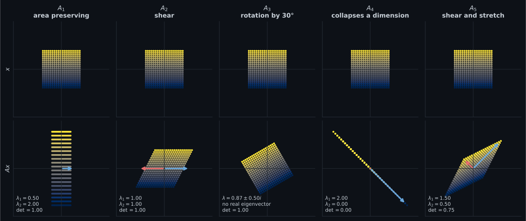
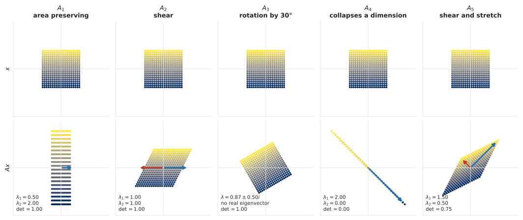
Reading the plot

From the five mappings. Every case in the table below is a real possibility you will meet, and the figure has one of each:

matrix	eigenvalues	determinant	what it does
$\mathrm{diag}(\tfrac12, 2)$	$0.5$, $2$	$1$	stretches one axis, compresses the other; area preserved
$\begin{bmatrix}1&\tfrac12\\0&1\end{bmatrix}$	$1$, $1$	$1$	a shear; one eigendirection, drawn twice in opposite directions
$\mathbf{R}(30°)$	$0.866 \pm 0.5i$	$1$	a rotation; no real eigenvectors, so none are drawn
$\begin{bmatrix}1&-1\\-1&1\end{bmatrix}$	$0$, $2$	$0$	collapses the plane onto a line; area zero
$\begin{bmatrix}1&\tfrac12\\\tfrac12&1\end{bmatrix}$	$0.5$, $1.5$	$0.75$	shear and stretch; symmetric, so the eigenvectors are orthogonal

The two to dwell on are the third and fourth. The rotation has determinant $1$ — it preserves area perfectly — and yet has no eigenvectors, which shows that “well behaved” and “has eigenvectors” are unrelated. The collapsing map has a zero eigenvalue, and a zero eigenvalue is exactly a nonzero vector in the kernel: $\mathbf{A}\mathbf{x} = 0\mathbf{x} = \mathbf{0}$. So $\lambda = 0$ appearing in a spectrum is the eigenvalue statement of singularity.

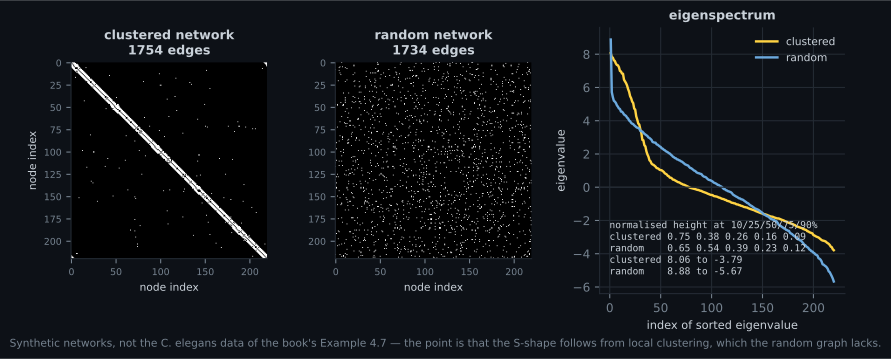
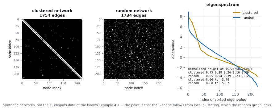
From the eigenspectrum. Both matrices are symmetrised as $\mathbf{A} + \mathbf{A}^\top$, exactly as the book does for the C. elegans connectivity matrix, and for exactly the reason the book gives: the raw connectivity matrix is not symmetric, so its eigenvalues need not be real. After symmetrising, Theorem 4.15 guarantees they are.

The shape measurement is the interesting part. Rescale each sorted spectrum to $[0,1]$ and read its height at fixed index fractions: the clustered network gives $0.75, 0.38, 0.26, 0.16, 0.09$ and the random one $0.65, 0.54, 0.39, 0.23, 0.12$. The random spectrum is close to a straight line; the clustered one falls off a cliff and then flattens. That knee is the book’s S-shape, and it comes from local clustering rather than from anything biological.

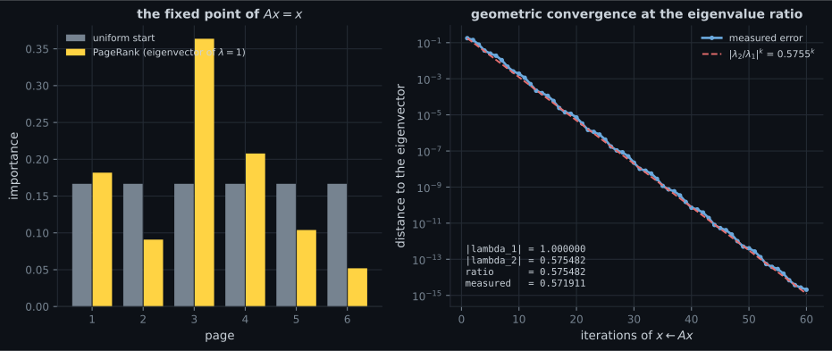
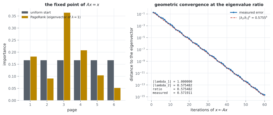
From PageRank. The bar chart is the fixed point of $\mathbf{A}\mathbf{x} = \mathbf{x}$: page 3 gets the most weight at $0.3636$ because everything links to it, and page 6 the least at $0.0519$. The book’s description is exact — the sequence $\mathbf{x}, \mathbf{A}\mathbf{x}, \mathbf{A}^2\mathbf{x}, \dots$ converges to an $\mathbf{x}^*$ with $\mathbf{A}\mathbf{x}^* = \mathbf{x}^*$, i.e. an eigenvector with eigenvalue $1$.

The right panel measures the rate. $\lvert\lambda_1\rvert = 1$ exactly (the matrix is column-stochastic, so it must be), $\lvert\lambda_2\rvert = 0.575482$, and the fitted decay rate over iterations $5$ to $35$ is $0.571911$. The error falls from $1.77\times10^{-1}$ at one iteration to $2.06\times10^{-15}$ at sixty.

That ratio is the whole story of why PageRank was practical: the number of iterations you need depends on the spectral gap, not on the size of the web. A gap of $0.575$ buys about one decimal digit every four iterations regardless of how many pages there are.

Pitfalls

Nobody computes eigenvalues from the characteristic polynomial

The polynomial is how the definition is stated. Finding its roots is badly conditioned — a tiny change in a coefficient can move a root enormously, and for a repeated root the sensitivity is worse still. The EigenLab stepper on this page has to cluster and polish its roots precisely because a double root lands about $10^{-8}$ off, and an eigenvalue $10^{-8}$ off makes $\mathbf{A}-\lambda\mathbf{I}$ nonsingular, which collapses the eigenspace to nothing and reports a diagonalisable matrix as defective. Real libraries use an iterative factorisation and never form the polynomial.

np.linalg.eig returns complex arrays, and eigvalsh lies about non-symmetric input

eig on a non-symmetric matrix returns complex128 even when every eigenvalue happens to be real, so downstream code that assumes floats breaks. eigh/eigvalsh are much faster and return real values — because they assume symmetry and read only the lower triangle. Handed a non-symmetric matrix they return confidently wrong answers with no warning. Check symmetry before choosing.

Geometric multiplicity is not numerically decidable

It is the nullity of $\mathbf{A}-\lambda\mathbf{I}$, and nullity needs a rank tolerance. The Eigendecomposition page measures matrices that are defective by construction and still get reported non-defective about $5\%$ of the time, because a badly conditioned conjugation makes the deficient eigenspace look full at any fixed tolerance. Treat “defective” as a statement about exact arithmetic, not about a float.

Eigenvector signs and orderings are conventions, not facts

Equation 4.26 says $c\mathbf{x}$ is an eigenvector whenever $\mathbf{x}$ is, so libraries pick a sign arbitrarily. The book’s own Remark adds that it does not assume eigenvalues are sorted, whereas numpy.linalg.eigh returns them ascending and eig returns them in no documented order. If your output depends on either — a PCA loading plot, a saved model, a regression test — impose your own convention.

A zero eigenvalue means singular; a small one does not mean nearly singular

$\lambda = 0$ is exactly a nonzero kernel vector, so it is equivalent to $\det\mathbf{A} = 0$. But eigenvalue magnitude is not a conditioning measure for a non-symmetric matrix: a matrix can have all eigenvalues of modulus $1$ and be arbitrarily ill conditioned. The right measure is the ratio of singular values, which is §4.5.

Symmetric matrices give orthogonal eigenvectors — but not the ones you computed

Example 4.8 is the trap. Its repeated eigenvalue has a genuinely two-dimensional eigenspace, and the natural basis for it that falls out of elimination is $\mathbf{x}_1^\top\mathbf{x}_2 = 1 \neq 0$ — not orthogonal. The spectral theorem promises an orthogonal basis exists; getting one requires Gram-Schmidt within each repeated eigenspace, licensed by Equation 4.40.

Compare

quantity	what it is	basis independent?	how many
eigenvalue	a scale factor $\lambda$ with $\mathbf{A}\mathbf{x} = \lambda\mathbf{x}$	yes	at most $n$ distinct
eigenvector	a direction the matrix only scales	no (it moves with the basis)	a whole line per eigenvalue, at least
eigenspace $E_\lambda$	$\ker(\mathbf{A}-\lambda\mathbf{I})$	as a subspace, yes	one per eigenvalue
algebraic multiplicity	root multiplicity in $p_{\mathbf{A}}$	yes	sums to exactly $n$ over $\mathbb{C}$
geometric multiplicity	$\dim E_\lambda$	yes	between $1$ and the algebraic multiplicity
eigenspectrum	the set of all eigenvalues	yes	—

pch.quizTag Check your understanding

1. Why does Definition 4.6 insist the eigenvector be nonzero?

   A For notational tidiness B Because A times the zero vector equals lambda times the zero vector for every lambda — without the exclusion, every number would be an eigenvalue of every matrix C Because the zero vector has no direction D Because the determinant would be zero
   pch.quizShowAnswer

   B — Because A times the zero vector equals lambda times the zero vector for every lambda — without the exclusion, every number would be an eigenvalue of every matrix — The same reason forces the eigenspace to be defined as the eigenvectors TOGETHER WITH zero: the eigenvectors alone are not a subspace, since they exclude the origin.

2. A 3x3 matrix has one eigenvalue with algebraic multiplicity 2 and geometric multiplicity 1, plus one simple eigenvalue. What follows?

   A It is diagonalisable B The eigenspace dimensions add to 2 out of 3, so there is no eigenbasis, the matrix is defective, and Theorem 4.20 will refuse to diagonalise it C Its determinant is zero D It has complex eigenvalues
   pch.quizShowAnswer

   B — The eigenspace dimensions add to 2 out of 3, so there is no eigenbasis, the matrix is defective, and Theorem 4.20 will refuse to diagonalise it — That is the book's Exercise 4.6(a) exactly: eigenvalues 1 (twice, one eigenvector) and 5. The geometric multiplicity can never exceed the algebraic one and here it is strictly less.

3. A rotation by 30 degrees has determinant 1 and no real eigenvectors. What does that combination show?

   A That the determinant was computed wrongly B That being well behaved and having eigenvectors are unrelated — the map is invertible, area-preserving and perfectly conditioned, and still fixes no direction, because its eigenvalues are the complex pair 0.866 plus or minus 0.5i C That rotations are singular D That the eigenvalues must be zero
   pch.quizShowAnswer

   B — That being well behaved and having eigenvectors are unrelated — the map is invertible, area-preserving and perfectly conditioned, and still fixes no direction, because its eigenvalues are the complex pair 0.866 plus or minus 0.5i — The determinant and trace theorems still hold: the conjugate pair multiplies to 1 and adds to 1.732, both real, because the imaginary parts cancel.

4. In the PageRank measurement, the error decays at 0.5719 per iteration against an eigenvalue ratio of 0.5755. What does that rate depend on?

   A The number of pages B The spectral gap — the ratio of the second-largest to the largest eigenvalue modulus — and not on the size of the graph at all C The starting vector D The number of links per page
   pch.quizShowAnswer

   B — The spectral gap — the ratio of the second-largest to the largest eigenvalue modulus — and not on the size of the graph at all — That independence from size is why the method scaled. A gap of 0.575 buys roughly one decimal digit every four iterations whether the graph has six nodes or six billion.

5. Theorem 4.14 says A-transpose A is symmetric and positive semidefinite for any A. Why does the chapter need that?

   A To compute determinants faster B Because it turns any matrix, of any shape, into a symmetric one — and the spectral theorem then gives that symmetric matrix a real orthonormal eigenbasis, which is exactly how section 4.5 constructs the SVD C Because it makes A invertible D To prove Theorem 4.12
   pch.quizShowAnswer

   B — Because it turns any matrix, of any shape, into a symmetric one — and the spectral theorem then gives that symmetric matrix a real orthonormal eigenbasis, which is exactly how section 4.5 constructs the SVD — Both halves are one line: symmetry from transposing the product, and semidefiniteness because x-transpose A-transpose A x is the squared length of Ax. Measured on a 2x3 matrix, the eigenvalues of A-transpose A come out 0, 1 and 6 — non-negative, with a zero because the rank is only 2.

🧪 Try It Yourself

Exercise 1 – Example 4.5 by hand

pch.exerciseTag pch.exerciseTitle

Exercise 2 – Algebraic against geometric multiplicity

pch.exerciseTag pch.exerciseTitle

Exercise 3 – The rotation has no real eigenvectors

pch.exerciseTag pch.exerciseTitle

Exercise 4 – Fix Example 4.8’s non-orthogonal eigenbasis

pch.exerciseTag pch.exerciseTitle

Exercise 5 – Power iteration and the spectral gap

pch.exerciseTag pch.exerciseTitle

Recall card

• An eigenvector is a nonzero direction the matrix only scales, and the eigenvalue is the scale factor. Every collinear vector is also an eigenvector, so an eigenvector is really a line.
• Four equivalent conditions: a nonzero solution of Ax = lambda x, a nontrivial null space for A minus lambda I, rank below n, determinant zero — which is why the eigenvalues are the roots of the characteristic polynomial.
• Algebraic multiplicity counts polynomial roots; geometric multiplicity is the eigenspace dimension. Geometric is at least one and never exceeds algebraic.
• A matrix is defective when the eigenspace dimensions add to less than n, and then no eigenbasis exists. Distinct eigenvalues are sufficient for a basis but not necessary.
• The spectral theorem is the result to remember: a symmetric matrix has real eigenvalues and an orthonormal eigenbasis — but not necessarily the basis you computed, so Gram-Schmidt within a repeated eigenspace may be needed.
• A-transpose A is symmetric and positive semidefinite for any A, which is how section 4.5 turns an arbitrary matrix into one the spectral theorem applies to.
• The determinant is the product of the eigenvalues and the trace is their sum, repeats included, and both hold for complex eigenvalues because conjugate pairs cancel.
• A rotation has no real eigenvectors despite being invertible and area-preserving, so being well behaved and having eigenvectors are unrelated.
• Never compute eigenvalues from the characteristic polynomial. Root-finding is badly conditioned, a double root lands about 1e-8 off, and an eigenvalue that far off destroys the eigenspace computation entirely.
• PageRank is the dominant eigenvector of a column-stochastic matrix, and power iteration converges at the spectral gap — measured 0.5719 against a predicted 0.5755, independent of graph size.

Next: Cholesky Decomposition — the first factorisation, and the one with the strictest hypothesis.