Updating the Means

With the responsibilities named, the first update falls out in half a page. §11.2.2 states it as a theorem and then spends the rest of the section on what it means — an importance-weighted average, an expectation, a picture of each data point tugging at each mean.

What you’ll learn

Theorem 11.1, Equation 11.20, and Example 11.3 reproduced: $-4 \to -2.701230$ , $0 \to -0.403411$ , $8 \to 3.704287$ , which round to the book’s $-2.7$ , $-0.4$ and $3.7$ .
Equation 11.23’s algebra: the stationarity condition is $\sum_n r_{nk}\mathbf{x}_n = N_k\boldsymbol\mu_k^{\text{new}}$ , checked to $1.8\times10^{-15}$ .
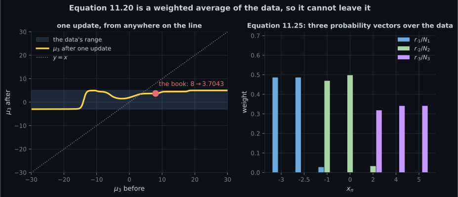
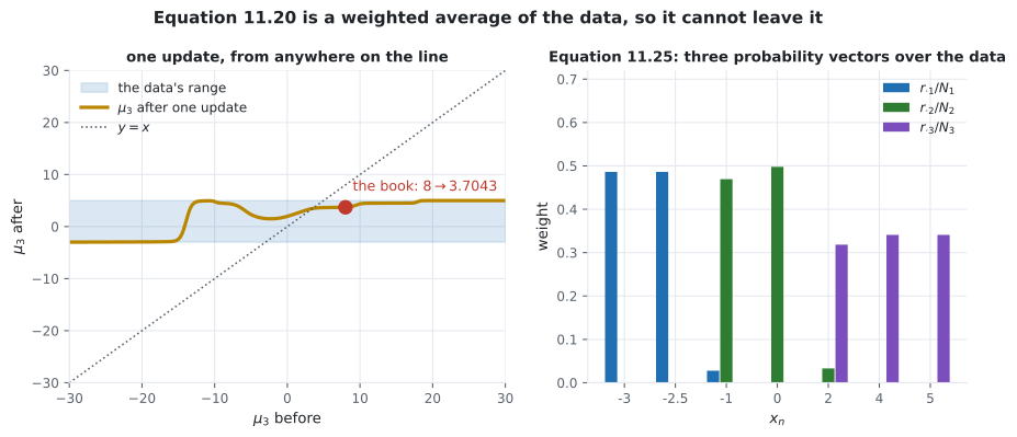
Equations 11.25–11.26, which say the update is literally an expected value — $\mathbf{r}_k$ is a probability vector over the data, verified to sum to $1$ exactly.
Why the update can never run away: $\boldsymbol\mu_k^{\text{new}}$ is a convex combination of the data, so one update lands every mean inside $[\min x, \max x]$ — the book’s $\mu_3$ goes from $8$ to $3.704287$ — and where that stops being true, at $\mu_3 = 73.585070$ , the component has died.
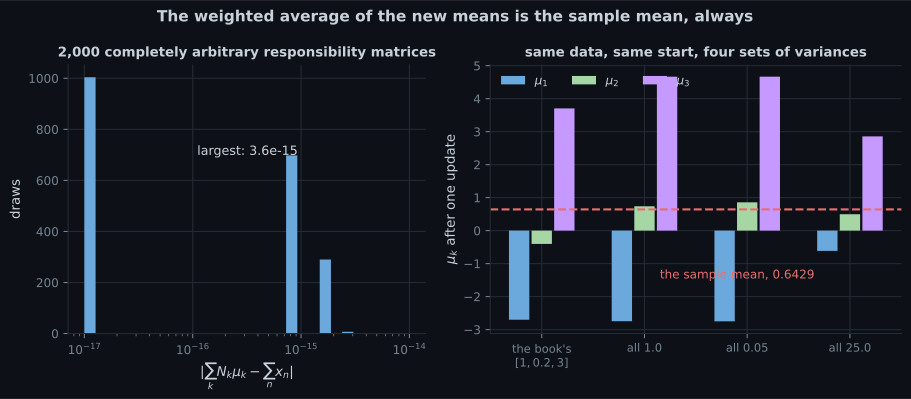
An invariant the book does not state: $\sum_k N_k\boldsymbol\mu_k^{\text{new}} = \sum_n \mathbf{x}_n$ exactly, for any responsibilities. Measured over $2000$ arbitrary matrices, worst error $3.6\times10^{-15}$ .
What one mean update alone buys: log-likelihood $-28.325536 \to -16.004150$ , a gain of $12.321385$ nats without touching a variance or a weight.
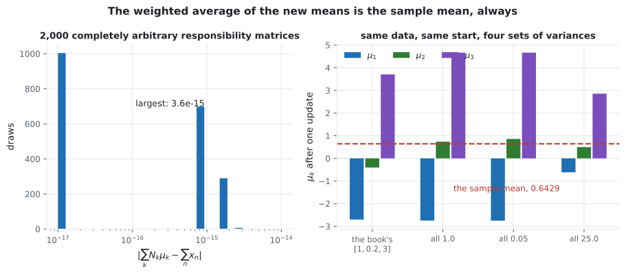
And the remark that follows the theorem: the same update with four different sets of variances gives four different answers.

Intuition: every mean is an average of the data, just not an equal one

The sample mean is $\frac{1}{N}\sum_n x_n$ — every point weighted $1/N$ . Equation 11.20 is the same formula with the weights changed: point $n$ gets weight $r_{nk}/N_k$ instead.

Everything else on this page follows from that single observation. The weights are non-negative and sum to one, so the answer is a convex combination: it lives inside the data, it cannot run off to infinity, and the arithmetic is a weighted average rather than anything more exotic. What makes the problem hard is not the formula — it is that the weights depend on the answer.

diagram One formula, three readings mermaid

  flowchart TD
  A["mu_k = (1/N_k) sum_n r_nk x_n
Equation 11.20"]
  A --> B["an importance-weighted
Monte Carlo estimate of the mean"]
  A --> C["E[X] under r_k = r_.k / N_k
Equations 11.25, 11.26"]
  A --> D["Figure 11.4: each point pulls
with strength r_nk"]
  B --> E["weights sum to 1 and are non-negative
-> mu_k lies inside the data"]
  C --> E
  D --> E

§11.2.2 Theorem 11.1

Theorem 11.1 (Update of the GMM Means). The update of the mean parameters $\boldsymbol\mu_k$ of the GMM is given by
$\boldsymbol\mu_k^{\text{new}} = \frac{\sum_{n=1}^{N} r_{nk}\mathbf{x}_n}{\sum_{n=1}^{N} r_{nk}} \qquad \text{(11.20)}$

The proof takes the derivative of Equation 11.21b through the chain rule, arrives at

\frac{\partial L}{\partial\boldsymbol\mu_k} = \sum_{n=1}^{N} r_{nk}(\mathbf{x}_n-\boldsymbol\mu_k)^\top\boldsymbol\Sigma_k^{-1} \qquad \text{(11.22c)}

and sets it to $\mathbf{0}^\top$ . Because $\boldsymbol\Sigma_k^{-1}$ is invertible it drops out entirely, leaving

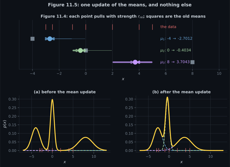
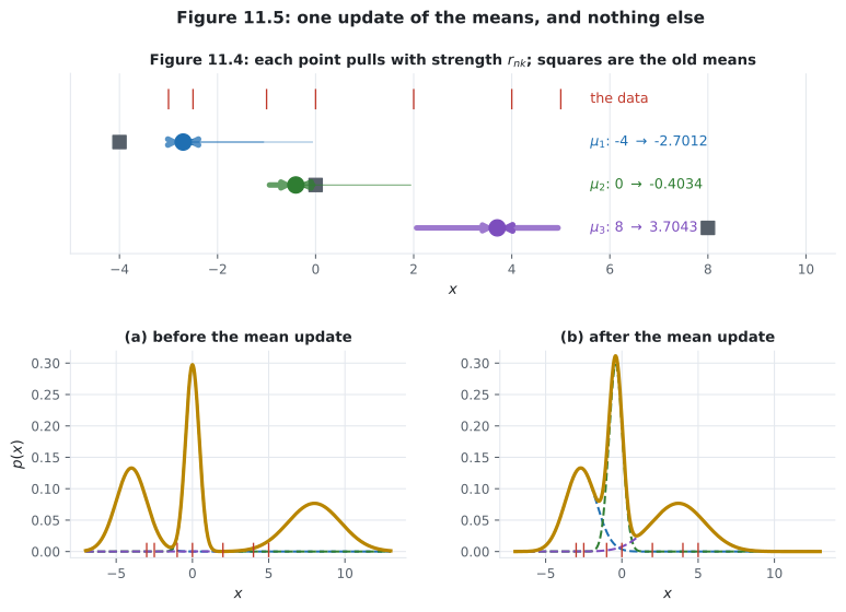
\sum_{n=1}^{N} r_{nk}\mathbf{x}_n = \sum_{n=1}^{N} r_{nk}\boldsymbol\mu_k^{\text{new}} = N_k\boldsymbol\mu_k^{\text{new}} \qquad \text{(11.23)}

Checked on the book’s initialisation:

	$k=1$	$k=2$	$k=3$
$\sum_n r_{nk}x_n$	$-5.555699$	$-0.810470$	$10.866169$
$N_k\mu_k^{\text{new}}$	$-5.555699$	$-0.810470$	$10.866169$

with a largest gap of $1.8\times10^{-15}$ , and

$k$	$\mu_k$ before	$\mu_k$ after	the book	$N_k$
$1$	$-4$	$\mathbf{-2.701230}$	$-2.7$	$2.057228$
$2$	$0$	$\mathbf{-0.403411}$	$-0.4$	$2.009008$
$3$	$8$	$\mathbf{3.704287}$	$3.7$	$2.933763$

Top, three horizontal tracks, one per component; on each, arrows of varying thickness run from the seven data points to a filled circle, with a grey square marking where the mean was. Bottom, two density plots side by side: before the update the three humps sit away from the data ticks, after it they sit on them. — Arrow thickness is the responsibility. The third component starts at 8 with no data anywhere near it, yet its responsibilities for the points at 2, 4 and 5 are 0.934, 1.000 and 1.000 — so it is pulled to 3.704287 in a single step. Nothing but the means changed between the two lower panels.

The same formula, said three ways

As an expectation. Define $\mathbf{r}_k := [r_{1k},\ldots,r_{Nk}]^\top / N_k$ (Equation 11.25). Then $\boldsymbol\mu_k \leftarrow \mathbb{E}_{\mathbf{r}_k}[\mathcal{X}]$ (Equation 11.26). Measured: each column of $\mathbf{r}_k$ sums to exactly $1$ , every entry is non-negative, and $\sum_n r_{nk}x_n$ under those weights reproduces Equation 11.20 to $8.9\times10^{-16}$ .

As importance weighting. “An importance-weighted Monte Carlo estimate of the mean, where the importance weights of data point $\mathbf{x}_n$ are the responsibilities $r_{nk}$ .”

As a picture. “The mean $\boldsymbol\mu_k$ is pulled toward a data point $\mathbf{x}_n$ with strength given by $r_{nk}$ .”

Left, a shaded horizontal band covering the data's range, with an S-shaped curve that leaves the diagonal and flattens inside the band at both ends, and a marked point at eight. Right, three groups of bars showing each component's weights over the seven data points. — The left panel runs the same single update with the third mean initialised anywhere from -30 to +30. Wherever it starts, one application of Equation 11.20 puts it inside the shaded band, because the update is an average of the data with non-negative weights summing to one. Past about 73.6 the component's total responsibility underflows to zero and the update stops being defined at all. The right panel is those weights.

Because $r_{nk}/N_k \geq 0$ and $\sum_n r_{nk}/N_k = 1$ :

\min_n x_n \ \leq\ \mu_k^{\text{new}} \ \leq\ \max_n x_n \qquad\text{whenever } N_k > 0

Measured over $4000$ starting values for $\mu_3$ spread across $[-40, 55]$ : zero excursions outside $[-3, 5]$ , worst deviation $0.0$ . A mean outside the data’s range means the responsibilities are wrong, not the update.

The proviso is not decoration. Push $\mu_3$ far enough away and every $r_{n3}$ underflows to exactly zero, so $N_3 = 0$ and Equation 11.20 is $0/0$ :

$\mu_3$ before	$N_3$	$\mu_3$ after
$8$	$2.934\times10^{0}$	$3.704287$
$30$	$1.292\times10^{-28}$	$5.000000$
$60$	$2.475\times10^{-202}$	$5.000000$
$\mathbf{80}$	$\mathbf{0}$	$\mathbf{\text{undefined}}$

Bisected, $N_3$ reaches exactly zero at $\mu_3 = 73.585070$ on the right and $-69.812512$ on the left. That is component death — the standard failure of EM in practice, and it is a genuine division by zero rather than a rounding problem: page 1103’s log-space form does not rescue it, because the quantity really is $0/0$ . Implementations guard it by re-seeding the component or flooring $N_k$ .

It is also the reason a badly initialised GMM recovers so fast in the first iteration and so slowly afterwards — the first step is a jump into the data, and page 1102 measured exactly that: $4.295713$ on round one, then $0.130775$ , then $0.018414$ .

An invariant the book does not state

Swap the order of summation in $\sum_k N_k\boldsymbol\mu_k^{\text{new}}$ :

\sum_{k}N_k\boldsymbol\mu_k^{\text{new}} = \sum_k\sum_n r_{nk}\mathbf{x}_n = \sum_n\mathbf{x}_n\underbrace{\sum_k r_{nk}}_{=\,1} = \sum_n \mathbf{x}_n

So after any mean update, $\frac{1}{N}\sum_k N_k\boldsymbol\mu_k = \bar{\mathbf{x}}$ , whatever the responsibilities were:

	value
$\sum_k N_k\mu_k^{\text{new}}$	$4.500000000000$
$\sum_n x_n$	$4.500000000000$
$\frac{1}{N}\sum_k N_k\mu_k$	$0.642857142857$
the sample mean $\bar{x}$	$0.642857142857$

Left, a log-scale histogram of two thousand values, all between 1e-17 and 4e-15. Right, four groups of three bars, visibly different between groups, with a dashed horizontal line marking 0.6429. — The left panel replaces the responsibilities with 2,000 random Dirichlet draws — matrices with no connection to the data or the model — and the identity still holds to 3.6e-15 every time. It is not a property of the fit; it follows only from each row summing to one.

What one update alone is worth

Freezing the variances and weights at the book’s initialisation and iterating only Equation 11.20:

round	log-likelihood	change	$\boldsymbol\mu$
$0$	$-28.325536$		$-4,\ 0,\ 8$
$1$	$-16.004150$	$\mathbf{+12.321385}$	$-2.7012,\ -0.4034,\ 3.7043$
$2$	$-15.965308$	$+0.038842$	$-2.5705,\ -0.4539,\ 3.6003$
$3$	$-15.964766$	$+0.000541$	$-2.5520,\ -0.4550,\ 3.5891$
$4$	$-15.964732$	$+0.000034$	$-2.5476,\ -0.4541,\ 3.5881$
$12$	$-15.964728$	$+0.000000$	$-2.5455,\ -0.4534,\ 3.5882$

Most negative single step over twelve rounds: $+0.0$ — the mean update alone never decreases the log-likelihood, which is the special case of §11.3’s guarantee. Note also where it stops: $-15.964728$ , well short of the full algorithm’s $-13.973323$ . The means alone cannot get there; the variances have to move too.

And the update still depends on everything

The remark right after Theorem 11.1: “the update of the means $\boldsymbol\mu_k$ […] depends on all means, covariance matrices $\boldsymbol\Sigma_k$ , and mixture weights $\pi_k$ via $r_{nk}$ . Therefore, we cannot obtain a closed-form solution for all $\boldsymbol\mu_k$ at once.”

Same data, same starting means, same weights — only the variances differ:

variances	$\boldsymbol\mu^{\text{new}}$
the book’s $[1, 0.2, 3]$	$-2.7012,\ -0.4034,\ 3.7043$
all $1.0$	$-2.7462,\ 0.7371,\ 4.6666$
all $0.05$	$-2.7500,\ 0.8571,\ 4.6667$
all $25.0$	$-0.6145,\ 0.4968,\ 2.8566$

The last row is the instructive one: with huge variances every component is nearly equally responsible for everything, so all three means collapse toward the sample mean $0.642857$ . The variances decide how sharply the data is divided, and the means only then decide where the pieces sit.

pch.quizTag Is the mean update clear?

In Equation 11.22c the inverse covariance appears. Why does it not appear in Equation 11.20?

pch.quizShowAnswer

B — Setting the gradient to zero lets an invertible matrix be cancelled from both sides — The stationarity condition becomes the sum of r times x equalling N_k times mu, with the inverse covariance multiplying both sides. That is why the mean update is a plain weighted average and carries no covariance in it — checked to 1.8e-15.
Why can a mean never leave the range of the data after one update?

pch.quizShowAnswer

B — The weights r_nk / N_k are non-negative and sum to one, so the update is a convex combination of the data — Measured: the book's third mean starts at 8 with no data beyond 5 and lands at 3.704287 in one step, and over four thousand starting values in [-40, 55] there are zero excursions outside [-3, 5]. The proviso is that N_k must be positive: past 73.585070 every responsibility underflows to zero and the update becomes 0/0.
What is the N_k-weighted average of the updated means?

pch.quizShowAnswer

B — Exactly the sample mean, for any responsibility matrix whatsoever — Swap the order of summation and the inner sum over k is one, leaving the sum of the data. Measured over 2,000 random Dirichlet matrices with no connection to the data, worst deviation 3.6e-15. So the mixture's overall mean is pinned to the data's after every M-step.
Iterating only the mean update, with variances and weights frozen, does what?

pch.quizShowAnswer

B — Increases it monotonically — plus 12.321385 on the first step — but stops at minus 15.964728, short of the full algorithm's minus 13.973323 — Most negative single step over twelve rounds: exactly zero. The means alone cannot reach the full optimum because the variances are what decide how sharply the data is divided — and with the variances fixed, the responsibilities can only move so far.

Exercises

Exercise 1 – Reproduce Example 11.3

Exercise 2 – A mean cannot leave the data

Exercise 3 – The update is an expectation

Exercise 4 – The invariant, on responsibilities from nowhere

Exercise 5 – The same update, four different answers

Recall card

Theorem 11.1: each mean becomes a responsibility-weighted average of the data, divided by that component’s total responsibility.
The inverse covariance in the gradient cancels, because setting an expression times an invertible matrix to zero removes the matrix. That is why the update carries no covariance.
Example 11.3 reproduced exactly: minus 4 to minus 2.701230, 0 to minus 0.403411, and 8 to 3.704287.
The update is literally an expectation, Equation 11.26, under a probability vector over the data built by normalising a column of responsibilities.
So every new mean is a convex combination of the data and cannot leave its range while its total responsibility is positive. Measured over four thousand starting values, zero excursions.
Which makes it a sanity check: a mean outside the data means the responsibilities are wrong, not the update.
Push a mean far enough away and its total responsibility underflows to exactly zero — at 73.585070 here — and the update becomes zero over zero. That is component death, and log-space arithmetic does not rescue it.
An invariant the book does not state: the N_k-weighted sum of the new means is the sum of the data, exactly, for any responsibility matrix at all.
Verified over two thousand random Dirichlet matrices, worst deviation 3.6e-15. It follows only from each row summing to one.
So the mixture’s overall mean is pinned to the sample mean after every M-step, and only the distribution of mass among components can move.
One mean update alone is worth 12.321385 nats on the book’s example, and iterating it never decreases the likelihood.
But it stalls at minus 15.964728, short of the full algorithm’s minus 13.973323 — the variances have to move too.
And the update depends on every other parameter: four sets of variances give four different answers from the same start, collapsing toward the sample mean when the variances are large.

Next: Updating the Covariances — §11.2.3, where the same argument runs again and the law of total variance from page 1101 comes back.

pch.coffeeTagline

pch.coffeeCta

pch.feedbackHeading

pch.feedbackSubheading