Evaluating Generative Models (FID, Coverage and Memorisation)

The GAN page needed an outside measurement to notice that eight of ten digit classes were missing, because no GAN loss can tell you that. This page builds the three measurements that generative work actually relies on, and then breaks each one on purpose — because a metric you cannot fool is a metric you have not tested.

The headline result is the second row from the bottom of this table. A “model” that simply repeats 200 real training images scores better than genuinely held-out real data on the Fréchet distance:

Sample source	Fréchet distance	Classes	KL from uniform	Judge confidence	Distance to nearest real image
Real, held out	9.605	10	0.0034	0.9942	5.3286
Blurred 5×5	25.142	10	0.0090	0.9248	4.7352
Noise added	37.717	10	0.2097	0.8802	5.0685
Only 5 of 10 classes	27.245	5	1.2223	0.9783	0.0024
200 images repeated	5.027	10	0.0430	0.9886	0.0022
Pure noise	643.959	3	11.1625	0.8239	15.1119

Read that row carefully: near-perfect distribution match, full class coverage, high classifier confidence — and it generated nothing. Only the last column notices.

What you’ll learn

• What the Fréchet distance actually computes, and why its floor is 9.605 here rather than zero.
• Why every FID number is meaningless without naming its feature extractor.
• Coverage, and why it catches the dropped-class failure (KL 1.2223) that the Fréchet distance ranks about the same as a blur.
• A memorisation check, and why the other two metrics cannot replace it.
• How the VAE and GAN from the previous pages score when all three are applied at once.

The Fréchet distance

FID fits one multivariate Gaussian to the real features and one to the generated features, then measures the distance between those two Gaussians in closed form:

$$d^2 = \lVert \mu_r - \mu_g \rVert^2 + \operatorname{tr}\!\left(\Sigma_r + \Sigma_g - 2\left(\Sigma_r \Sigma_g\right)^{1/2}\right)$$

The first term compares the average feature; the second compares how features co-vary. In one dimension it collapses to something you can check by hand — $(\mu_r - \mu_g)^2 + (\sigma_r - \sigma_g)^2$ — which is exactly what the sketch below does.

The Frechet distance between two feature sets

from scipy import linalg
 
features_real = extractor.predict(real_images)
features_fake = extractor.predict(generated_images)
 
mu_r, mu_g = features_real.mean(axis=0), features_fake.mean(axis=0)
cov_r = np.cov(features_real, rowvar=False)
cov_g = np.cov(features_fake, rowvar=False)
 
covmean, _ = linalg.sqrtm(cov_r @ cov_g, disp=False)
if np.iscomplexobj(covmean):          # sqrtm returns complex from rounding
    covmean = covmean.real
 
distance = ((mu_r - mu_g) ** 2).sum() + np.trace(cov_r + cov_g - 2 * covmean)

Two details matter more than the formula.

The features are the metric. Published FID numbers use a specific Inception network trained on ImageNet. There is no such cached model on this machine, so these features come from a classifier trained here on the same data, reaching 0.9477 validation accuracy. That is a legitimate Fréchet distance in this feature space, and it is not comparable with any published FID. Neither are two published numbers from different extractors.

There is a floor, and it is not zero. Two disjoint samples of real MNIST score 9.605, because 2,000 samples cannot estimate a 64-dimensional covariance exactly. A model scoring 9.605 has matched the data as well as the data matches itself. Reporting a distance without that reference makes any number unreadable.

Each metric, deliberately broken

figure 2,000 samples per source, same feature extractor throughout matplotlib

The two panels disagree about which failure is worse, which is the point. The Frechet distance ranks 'only 5 of 10 classes' (27.245) as barely worse than a 5x5 blur (25.142), while coverage separates them by two orders of magnitude — 1.2223 against 0.0090. And the repeated-images row beats real held-out data on the left panel (5.027 against 9.605) while looking perfect on the right.

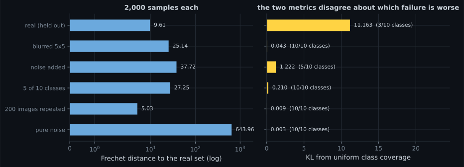
Working through the rows:

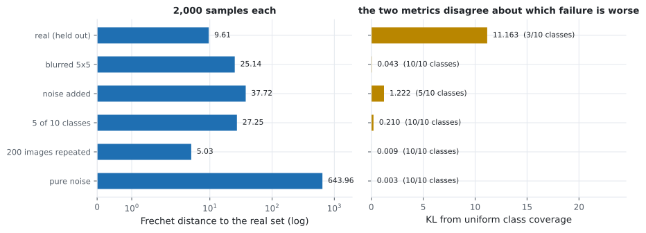
• Blur damages every feature a little. The Fréchet distance rises to 25.142 and coverage barely moves (0.0090) — a blurred 7 is still classified as a 7.
• Added noise scores worse than blur on the Fréchet distance (37.717) and starts to disturb coverage (0.2097).
• Dropping five classes is the failure GANs actually exhibit. Coverage catches it immediately (5 classes, KL 1.2223). The Fréchet distance registers 27.245, which on its own would read like a mild quality problem rather than half the dataset missing.
• Repeating 200 real images is the adversarial case. Every image is real, so the feature statistics are close to correct — 5.027, below the held-out floor. Coverage is fine, 10 classes. Judge confidence is 0.9886.
• Pure noise is the sanity check every metric must pass: 643.959, and 3 classes at KL 11.1625.

Note the confidence column across all of it. The five-class row scores 0.9783, higher than real held-out data’s own blurred version — because a classifier is confident about the classes that are present and is never asked about the ones that are not. Confidence measures sharpness, never diversity.

Coverage

Coverage needs a labeller, not a distance. Classify every sample, then compare the resulting class distribution against the one you wanted:

$$D_{\mathrm{KL}}(u \,\|\, p) = \sum_{c} u_c \log \frac{u_c}{p_c}, \qquad u_c = \tfrac{1}{10}$$

The direction matters, and it is measurable. With uniform $u$ on the left, any class the model never produces sends the term to infinity — so the shares are clipped away from zero, and a missing class becomes a large finite penalty. Reverse the arguments and the metric saturates:

Class distribution	$D_{\mathrm{KL}}(u \,\|\, p)$	$D_{\mathrm{KL}}(p \,\|\, u)$
Near-uniform	0.0015	0.0015
Five classes, evenly	8.8638	0.6931 = $\log 2$
One class only	16.3484	2.3026 = $\log 10$

The reversed direction cannot exceed $\log 10 = 2.3026$ no matter how badly the model collapses, because a distribution concentrated on one class is perfectly “explained” by itself. The correct direction grows without bound as classes disappear, which is exactly the behaviour coverage needs.

diagram Diagram mermaid

  flowchart TD
  S["generated samples"] --> F["feature extractor"]
  S --> J["judge classifier"]
  S --> N["nearest-neighbour search
against held-out real data"]
  F --> FID["Frechet distance
floor 9.605"]
  J --> COV["class coverage
KL from uniform"]
  N --> MEM["memorisation
distance to nearest real image"]
  FID -.->|"fooled by copying: 5.027"| X["needs the other two"]
  COV -.->|"fooled by copying: 10 classes"| X
  MEM -.->|"catches copying: 0.0022"| Y["the check nobody runs"]

Memorisation

The third measurement is the cheapest and the most often skipped: for each generated sample, find the nearest real image in a held-out split and report the distance.

Memorisation, in one distance matrix

squared = (np.sum(samples ** 2, axis=1)[:, None]
           + np.sum(reference ** 2, axis=1)[None, :]
           - 2 * samples @ reference.T)
nearest = np.argmin(squared, axis=1)
distance = np.sqrt(np.maximum(squared[np.arange(len(samples)), nearest], 0))

Two things about the reference set are not optional.

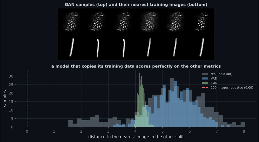
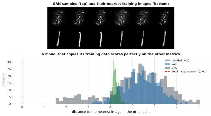
It must be disjoint from the samples being scored. My first version of this table compared the real baseline against the split it was drawn from, so every image found itself and the row read 0.0031 — a number that looks like catastrophic copying and is really a self-match. Scoring every row against the test split instead gives 5.1825 for real data, which is the honest floor.

And the comparison must be against data the model trained on if what you want to detect is training-set memorisation. Those are two different questions — “is this a copy of something real” and “is this a copy of something it was shown” — and only the second is a legal or licensing concern.

figure Distance to the nearest image in the other split matplotlib

The three distributions overlap, which is the desired result: none of these models is copying. The dashed line is where the repeated-images source lands, at 0.0022 — three orders of magnitude away from every genuine model. This is a check with an unambiguous reading, which is rare among generative metrics.

The three models, scored together

figure Same feature extractor, same judge, same reference split matplotlib

The VAE lands close to the real-data floor on every axis — Frechet 17.165 against 9.605, coverage KL 0.0534 against 0.0034 — while the GAN's 306.752 and KL 13.0709 record the mode collapse the GAN page measured. Both have nearest-neighbour distances in the same range as real held-out data (5.3754 and 4.2331 against 5.1825), so neither is memorising.

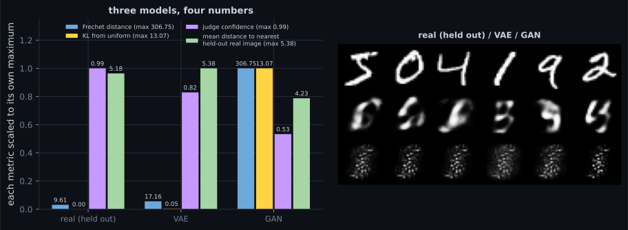
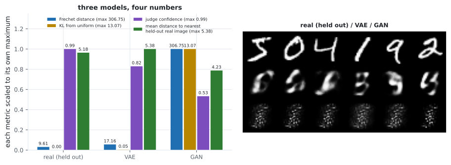
Model	Fréchet	Classes	KL from uniform	Judge confidence	Nearest held-out real image
Real, held out	9.605	10	0.0034	0.9942	5.1825
VAE	17.165	10	0.0534	0.8244	5.3754
GAN	306.752	2	13.0709	0.5302	4.2331

The VAE is 7.560 above the floor and the GAN is 297.147 above it. Stated as a ratio the GAN looks 18× worse than the VAE, and as a distance above the floor it looks 39× worse — which is a good reminder that the Fréchet distance is not on a scale where ratios mean anything. What survives either reading is the ordering, and the ordering agrees with coverage.

sketch The Frechet distance in one dimension p5.js Pause Restart

Drag either curve's centre to move its mean, or its slider to change its width. The distance is the closed-form value, so you can see which term is doing the work.

What to report

A defensible evaluation of a generative model is short:

1. The Fréchet distance, with its floor. Score two disjoint samples of real data through the identical pipeline and publish that number next to the model’s. Here: 9.605.
2. Coverage against a stated target. Classes produced and KL from the target distribution. Say what the labeller is and how accurate it is (0.9477 here).
3. Nearest-neighbour distance to a disjoint real split. With the same number for real data as the reference (5.1825).
4. The feature extractor, named. Without it the first number means nothing.
5. Uncurated samples. A fixed noise batch, not a selection.

Anything missing from that list is a place a result can hide.

sketch The measured table, ranked p5.js Pause Restart

Click a column to rank every row by it. The bars are that column's values and the highest and lowest are computed from the numbers, not written in.

Pitfalls

• Reporting a Fréchet distance without its floor. 9.605 was as good as real data got here; a model at 17.165 is close, not broken.
• Comparing FID across papers or feature extractors. These numbers come from a locally trained 0.9477-accuracy classifier and are not comparable with Inception-based FID at all.
• Using the Fréchet distance alone. Repeating 200 real images scored 5.027, better than the real-data floor, while generating nothing.
• Using coverage alone. The repeated-images source covered all 10 classes at KL 0.0430.
• Reading judge confidence as quality. The five-class source scored 0.9783 while missing half the data.
• Scoring memorisation against the split the samples came from. That produced 0.0031 for real data — a self-match that looks like copying. Use a disjoint split; the honest floor was 5.1825.
• Estimating a covariance from too few samples. The floor rises as the sample count falls, so every number in a comparison must use the same count.

Recap

• The Fréchet distance compares two Gaussians fitted in a feature space; its value depends entirely on that feature space, and its floor here is 9.605, not 0.
• Coverage needs a labeller and a stated target; KL from uniform caught the dropped-class failure at 1.2223 where the Fréchet distance read 27.245, similar to a blur’s 25.142.
• Memorisation needs a nearest-neighbour search against a disjoint real split. Repeated images scored 0.0022 against 5.1825 for genuine data.
• Copying the training set defeats both distribution metrics simultaneously — 5.027 and 10 classes — so the third check is not optional.
• Judge confidence measures sharpness only. It was 0.9886 for the copied set and 0.9783 for the half-missing set.
• Scored together: VAE 17.165 / 10 classes / KL 0.0534, GAN 306.752 / 2 classes / KL 13.0709, neither memorising.

Next

With measurement settled, the remaining generative families can be judged rather than admired. Next is the one that turns a fixed noise schedule into a generator: Diffusion Models (Introduction).

pch.quizTag pch.quizDefaultTitle

1. A source that simply repeats 200 real training images scored a Frechet distance of 5.027, while genuinely held-out real data scored 9.605. What does that show?

   A The repeated images are higher quality than real data B The Frechet distance cannot detect memorisation — copying real data reproduces its feature statistics almost exactly, so the metric rewards it C The feature extractor was broken D 2,000 samples is too few to compute the metric
   pch.quizShowAnswer

   B — The Frechet distance cannot detect memorisation — copying real data reproduces its feature statistics almost exactly, so the metric rewards it — It is a distribution distance, and a subset of the real distribution is a very good match to it. Only a nearest-neighbour check noticed, at 0.0022.

2. Why is the Frechet distance between two disjoint samples of real data 9.605 rather than 0?

   A The metric is miscalibrated B Because 2,000 samples cannot estimate a 64-dimensional mean and covariance exactly, so finite-sample error sets a floor that must be reported alongside any model's score C Because the two samples come from different distributions D Because the feature extractor is only 0.9477 accurate
   pch.quizShowAnswer

   B — Because 2,000 samples cannot estimate a 64-dimensional mean and covariance exactly, so finite-sample error sets a floor that must be reported alongside any model's score — The floor moves with the sample count, which is why every model in a comparison must be scored with the same number of samples.

3. A source containing only 5 of the 10 digit classes scored 27.245 on the Frechet distance and 1.2223 on coverage KL, while a 5x5 blur scored 25.142 and 0.0090. What is the lesson?

   A Blur is worse than dropping classes B The Frechet distance ranks the two failures as roughly equal while coverage separates them by two orders of magnitude — the metrics answer different questions and you need both C Coverage is the only metric worth computing D The judge classifier was too weak
   pch.quizShowAnswer

   B — The Frechet distance ranks the two failures as roughly equal while coverage separates them by two orders of magnitude — the metrics answer different questions and you need both — A distribution distance in feature space is dominated by per-sample quality; whether a whole mode is missing needs an explicit class-level measurement.

4. The memorisation check first reported 0.0031 for real held-out data, suggesting near-perfect copying. What was wrong?

   A The real data was corrupted B The samples were drawn from the same split used as the reference, so every image found itself; scoring against a disjoint split gave the honest floor of 5.1825 C The distance formula was missing a square root D The sample count was too low
   pch.quizShowAnswer

   B — The samples were drawn from the same split used as the reference, so every image found itself; scoring against a disjoint split gave the honest floor of 5.1825 — A nearest-neighbour check is only meaningful against data the scored samples are not part of.

5. Why must a reported FID always name its feature extractor?

   A For reproducibility paperwork only B Because the number is a distance in that network's feature space — the features here come from a locally trained 0.9477-accuracy classifier, so the values are not comparable with published Inception-based FID C Because Inception is proprietary D It does not matter as long as the same data is used
   pch.quizShowAnswer

   B — Because the number is a distance in that network's feature space — the features here come from a locally trained 0.9477-accuracy classifier, so the values are not comparable with published Inception-based FID — Different extractors give different geometries, so two FID numbers from different pipelines cannot be ranked against each other at all.

🧪 Try It Yourself

pch.exerciseTag pch.exerciseTitle

pch.exerciseTag pch.exerciseTitle

pch.exerciseTag pch.exerciseTitle

pch.exerciseTag pch.exerciseTitle

pch.exerciseTag pch.exerciseTitle

pch.exerciseTag pch.exerciseTitle