Sequence-to-Sequence Learning (Machine Translation)

Every model so far has read a sequence and produced a label. Translation, summarisation and normalisation produce a sequence — of a different length, in a different vocabulary, with a different order. That needs two networks: an encoder that reads and a decoder that writes.

The task here is date normalisation with the date buried in filler: order 21 item 45 07/02/1993 id seq → 1993-02-07. Real translation corpora are large downloads; this one is generated, so the alignment is known exactly and an attention map can be checked rather than admired.

Model	Parameters	Teacher-forced	Free-running character	Free-running exact
encoder–decoder	70,156	0.9616	0.9217	0.6250
+ attention	70,924	0.9979	0.9957	0.9770

768 extra parameters — 1.1% — took exact match from 0.6250 to 0.9770.

What you’ll learn

The encoder–decoder shape, and why the decoder needs its own input.
Teacher forcing, and the gap it hides: 0.0399 character accuracy for the attention-free model against 0.0022 with attention.
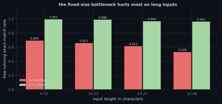
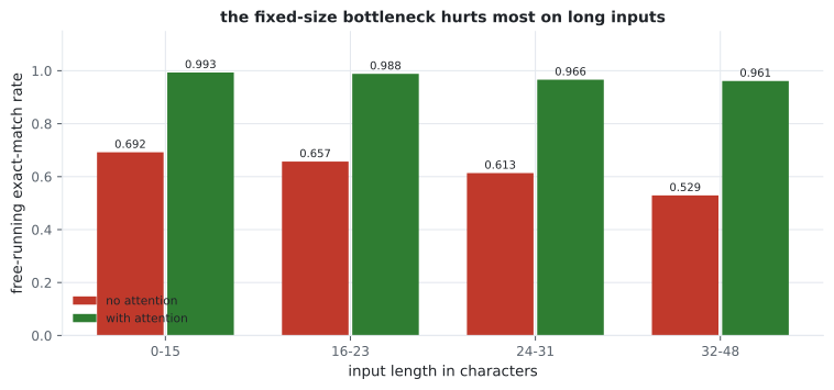
Why a single fixed-size state is a bottleneck, measured by input length: exact match falls 0.6921 → 0.5291 without attention and 0.9934 → 0.9612 with it.
How to read an attention matrix when you know the true alignment.
Greedy decoding, and where beam search would help.

The shape

Encoder to decoder, with the state as the bridge

encoder_inputs = keras.layers.Input((INPUT_LENGTH,))
embedded = keras.layers.Embedding(input_alphabet, WIDTH, mask_zero=True)(encoder_inputs)
encoder_sequence, state_h, state_c = keras.layers.LSTM(
    WIDTH, return_sequences=True, return_state=True)(embedded)
 
decoder_inputs = keras.layers.Input((OUTPUT_LENGTH,))
decoder_embedded = keras.layers.Embedding(output_alphabet, WIDTH)(decoder_inputs)
decoder_sequence = keras.layers.LSTM(WIDTH, return_sequences=True)(
    decoder_embedded, initial_state=[state_h, state_c])          # <- the bridge
 
outputs = keras.layers.Dense(output_alphabet, activation="softmax")(decoder_sequence)

Without attention, everything the decoder knows about the input is those two state vectors — 64 numbers each. The input can be 48 characters long. That is the bottleneck the rest of this page measures.

Teacher forcing, and what it hides

During training the decoder is fed the correct previous character, not its own prediction:

text

input:   \t 1 9 9 3 - 0 2 - 0
target:   1 9 9 3 - 0 2 - 0 7

This is teacher forcing, and it exists because it makes training parallel — every output position is computed at once, from known inputs. At inference there is no correct previous character, so the decoder consumes its own output and any error compounds. That mismatch is exposure bias.

Model	Teacher-forced	Free-running character	Cost of the mismatch
encoder–decoder	0.9616	0.9217	−0.0399
+ attention	0.9979	0.9957	−0.0022

Two panels. Left: grouped bars for both models showing teacher-forced accuracy, free-running character accuracy and free-running exact match — the attention-free model reads 0.962, 0.922 and 0.625 while the attention model reads 0.998, 0.996 and 0.977. Right: teacher-forced validation accuracy per epoch, where the attention model rises quickly above 0.99 and the attention-free one plateaus near 0.96. — The three bars per model are the same predictions scored three ways, and the spread between them is the point. Teacher-forced accuracy flatters both models — it is measured with the correct history handed to the decoder at every step. Free-running character accuracy is the honest per-character number, and exact match is what a user experiences: one wrong character makes the whole date wrong, so 0.9217 character accuracy becomes 0.6250 exact.

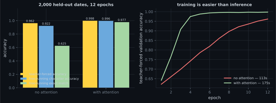
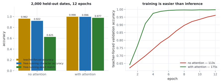
Note how much worse exact match is than character accuracy: 0.9217 per character becomes 0.6250 per date. With ten output characters, even independent errors compound — $0.9217^{10} \approx 0.44$ — and the measured 0.6250 is better than that only because the errors are correlated.

The bottleneck, by input length

Input length	Rows	Encoder–decoder	+ attention
0–15	302	0.6921	0.9934
16–23	685	0.6569	0.9883
24–31	652	0.6135	0.9663
32–48	361	0.5291	0.9612

Grouped bars of free-running exact-match rate by input length. Without attention the rate falls steadily from 0.6921 for short inputs to 0.5291 for the longest. With attention it stays between 0.9934 and 0.9612 across all four length bands. — The attention-free model loses 0.1630 from the shortest band to the longest; the attention model loses 0.0322. This is the fixed-size bottleneck made visible — two 64-number vectors have to carry a 48-character input, and the longer the input the less of it survives. Attention removes the constraint by letting the decoder look back at every encoder position directly, which is why the 1980s encoder-decoder became the 2015 attention model and then the transformer.

Reading the alignment

The task has a known alignment: the 1993 in the output comes from the 1993 in the input, and the day and month are reordered around it. So the attention matrix is checkable.

A heat map with input characters of 'order 21 item 45 07/02/1993 id seq' along the x axis and output characters of '1993-02-07' down the y axis. Bright cells appear where each output digit is generated: the year digits attend to the 1993 region, the month digits to the 02, and the day digits to the 07, with the filler words almost entirely dark. — Every bright cell is where it should be. The year characters attend to '1993', the month characters to '02', the day characters to '07' — and the filler words 'order', 'item', 'id', 'seq' are almost completely dark, including the distractor numbers 21 and 45. The two hyphens attend to the start of the input, which is a reasonable place to put 'I am emitting punctuation now'. This is the clearest interpretability result in the module, and it is only checkable because the corpus was generated with a known alignment.

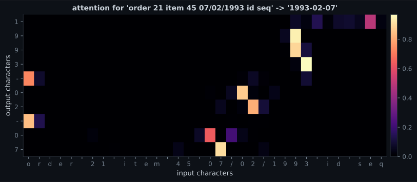
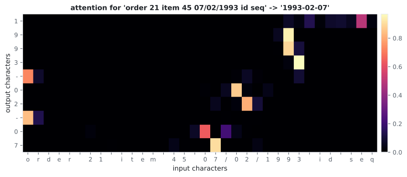
Compare that with the Grad-CAM page, where the trained and untrained heat maps still correlated at 0.6729. Here the alignment is verifiable against ground truth, so the attention map is evidence rather than decoration.

Greedy decoding, and its limits

Free-running decode, one character at a time

decoder_input = np.zeros((rows, OUTPUT_LENGTH), "int32")
decoder_input[:, 0] = start_token
for position in range(OUTPUT_LENGTH - 1):
    predictions = model.predict([x, decoder_input], verbose=0)
    decoder_input[:, position + 1] = predictions[:, position].argmax(axis=-1)

This takes the most likely character at each step and never reconsiders. It is what produced every number on this page, and it has a known weakness: an early high-confidence mistake cannot be undone, because the model conditions on it forever afterwards.

Beam search keeps the k best partial sequences instead of one, so a locally attractive wrong turn can lose to a globally better path. It costs k times the compute and matters most where this task is easy: long outputs with many plausible continuations — translation, summarisation — rather than a ten-character date with rigid grammar.

diagram Diagram mermaid

  flowchart LR
  A["input sequence"] --> B["encoder LSTM"]
  B --> C["final state
(2 x 64 numbers)"]
  B --> D["all encoder outputs
(48 x 64)"]
  C --> E["decoder LSTM"]
  D -. "attention only" .-> F["context vector
per output step"]
  E --> F
  F --> G["Dense softmax"]
  E --> G
  H["no attention:
exact 0.6250"] -.-> C
  I["with attention:
exact 0.9770"] -.-> D

sketch The bottleneck and the fix p5.js

Drag the input length. Without attention the decoder sees a fixed-size summary; with attention it sees every position. The exact-match numbers are the measured ones.

sketch The measured table, ranked p5.js

Click a column to rank every row by it. The bars are that column's values and the highest and lowest are computed from the numbers, not written in.

Pitfalls

Reporting teacher-forced accuracy as the model’s accuracy. It was 0.9616 against a free-running 0.9217 — and 0.6250 exact.
Reporting character accuracy for a task with a whole-output answer. 0.9217 per character is 0.6250 per date.
Omitting attention on any input longer than a few tokens. 768 extra parameters bought +0.3520 exact match.
Testing only on short inputs. The attention-free model lost 0.1630 from the shortest band to the longest; a short-input benchmark would have hidden it.
Forgetting the start token. The decoder input is the target shifted right behind a start symbol; get the shift wrong and the model learns to copy its input.
Trusting an attention map without a known alignment. Here it is checkable; on real data it usually is not.
Reaching for beam search first. It costs k× the compute and would not fix a bottleneck — attention would.

Recap

An encoder–decoder passes its final state as the bridge: without attention that is 64+64 numbers for an input up to 48 characters.
Teacher forcing makes training parallel and hides exposure bias — measured at 0.0399 character accuracy for the attention-free model, 0.0022 with attention.
Attention took free-running exact match from 0.6250 to 0.9770 for 768 extra parameters.
Exact match by input length: 0.6921 → 0.5291 without attention, 0.9934 → 0.9612 with.
The attention map matches the known alignment exactly — year to year, month to month, filler dark.
Greedy decoding cannot revisit an early mistake; beam search can, at k× the cost.

That closes the NLP phase. The same encoder–decoder shape reappears immediately in generative modelling, this time with a probabilistic middle: Phase 6 — Generative Deep Learning.

pch.quizTag pch.quizDefaultTitle

The attention-free model scored 0.9616 teacher-forced, 0.9217 free-running per character, and 0.6250 exact. Which number should be reported?

pch.quizShowAnswer

B — The exact-match rate — it is what a user experiences, and the other two flatter the model: teacher forcing hands the decoder the correct history, and per-character accuracy ignores that one wrong character ruins the whole date — With ten output characters, 0.9217 per character would give about 0.44 exact if errors were independent; the measured 0.6250 is higher only because they are correlated.
What is exposure bias, and how large was it here?

pch.quizShowAnswer

B — The mismatch between training on correct previous characters and inferring from its own outputs — measured at 0.0399 character accuracy without attention and 0.0022 with it — Attention shrinks it because the decoder can re-read the input at every step instead of relying on a state that its own earlier mistakes have corrupted.
Adding attention cost 768 parameters (1.1%) and raised exact match from 0.6250 to 0.9770. What was the bottleneck it removed?

pch.quizShowAnswer

B — Everything the decoder knew about the input was two 64-number state vectors, regardless of whether the input was 10 or 48 characters — attention lets it read every encoder position directly — The length breakdown shows it: the attention-free model lost 0.1630 from the shortest band to the longest, the attention model 0.0322.
Why is this page's attention map stronger evidence than a Grad-CAM heat map?

pch.quizShowAnswer

B — Because the corpus was generated with a known alignment, so the map can be checked against ground truth — the year characters really should attend to the year digits — The Grad-CAM page measured a 0.6729 correlation between trained and untrained maps. Here the filler words and distractor numbers are dark and the date regions are bright, which is a verifiable claim.
When is beam search worth its k-times compute cost?

pch.quizShowAnswer

B — When outputs are long and many continuations are plausible, so an early locally-attractive mistake can lose to a globally better path — not on a ten-character date with rigid grammar — Beam search would not have fixed the bottleneck measured here; attention did. Fix the architecture before the search.

🧪 Try It Yourself

pch.coffeeTagline

pch.coffeeCta

pch.feedbackHeading

pch.feedbackSubheading