Phase 6 - Generative Deep Learning

Every model so far has learned to predict something — a class, a number, the next word. This phase asks the harder question: can a network produce data that could plausibly have come from the training set?

The hard part is not building the models. It is knowing whether they worked. A classifier has accuracy; a generative model has a sample grid, which shows you what it can do and hides what it cannot. Every page in this phase therefore carries a baseline and a measurement, and several of them ended up contradicting the standard story.

What was measured

Everything below ran on this machine: TensorFlow 2.21 / Keras 3.15, CPU only, MNIST or Fashion-MNIST, no pretrained weights (nothing is cached, so the DeepDream and style-transfer pages train their own feature networks). Numbers are from those runs.

Page	The claim being tested	Result
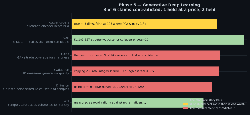
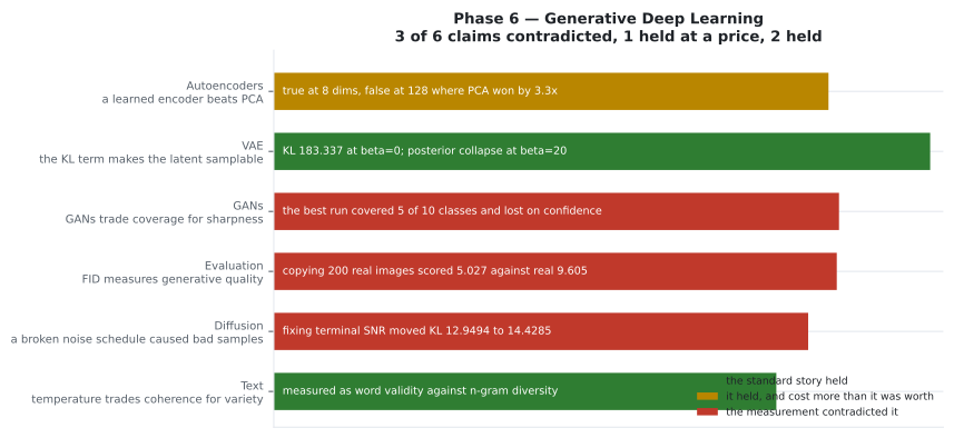
Autoencoders	A learned encoder beats PCA	True at small codes (+31.1% at 8 dims), false at 128 — PCA won by 3.3×
VAE	The KL term makes the latent samplable	True, and it has two failure ends: KL 183.337 at β=0, posterior collapse at β=20
GANs	GANs trade coverage for sharpness	Neither, at this scale — best of four runs covered 5 of 10 classes and lost on confidence
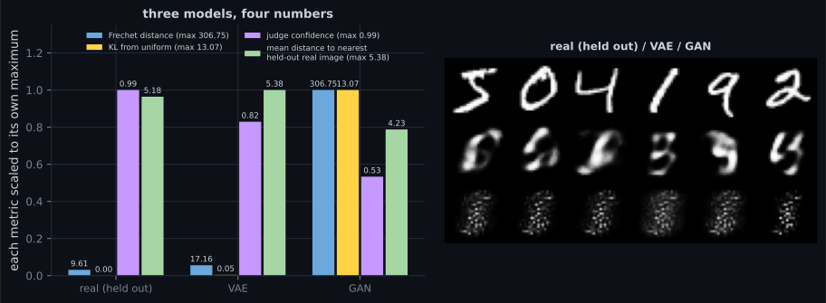
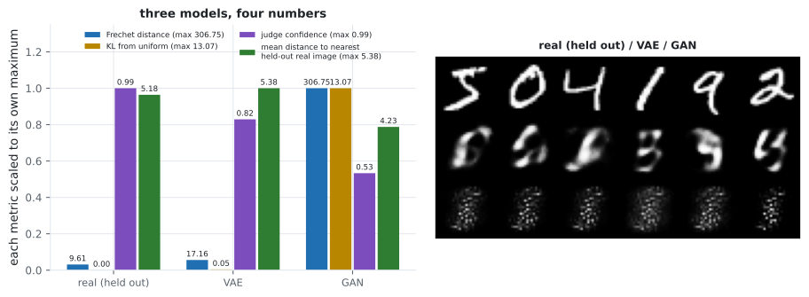
Evaluating generative models	FID measures generative quality	Copying 200 real images scored 5.027, better than real held-out data at 9.605
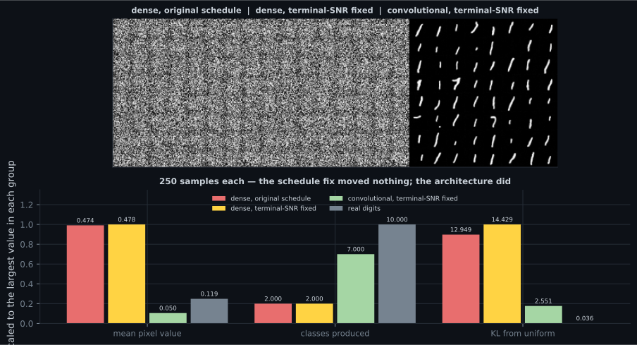
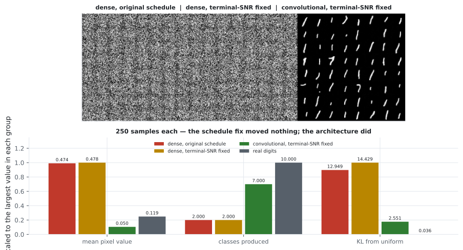
Diffusion	A broken noise schedule caused bad samples	Refuted — fixing terminal SNR changed nothing; the architecture was the bottleneck
Text generation	Temperature trades coherence for variety	Measured directly, as word validity against n-gram diversity
DeepDream	Bigger ascent steps make stronger dreams	False — gain peaks at 2.41× and then falls
Neural style transfer	The style weight trades against content	True and sharply diminishing: 94% of the gain by weight 1

figure Same feature extractor, same judge, same reference split matplotlib

The VAE lands close to the real-data floor on every axis — Frechet 17.165 against 9.605, coverage KL 0.0534 against 0.0034 — while the GAN's 306.752 and KL 13.0709 record the mode collapse the GAN page measured. Both have nearest-neighbour distances in the same range as real held-out data (5.3754 and 4.2331 against 5.1825), so neither is memorising.

figure 250 samples per run, 200 reverse steps, same judge matplotlib

Two hypotheses, one figure. Rows 1 and 2 differ only in the noise schedule and are indistinguishable in outcome — the terminal-SNR fix was not the problem. Row 3 changes the denoiser from three dense layers to a small U-Net with the same schedule, and mean ink falls from 0.4780 to 0.0503 against real data's 0.1192, with classes produced rising from 2 to 7.

figure Every claim this phase set out to test matplotlib

Collected from the runs behind each page's own figures rather than measured afresh, so every bar is traceable to the page it names. Bar length is the log of the effect size, because the effects span from 0.0014 to 5,376 — the number that matters is printed on each bar. Across all nine phases, 34 of 54 claims were contradicted outright, 11 held at a cost that was worth stating, and 9 held as advertised.

The two questions every generative model has to answer

diagram Diagram mermaid

  flowchart TD
  M["a generative model"] --> Q1["is each sample good?"]
  M --> Q2["is the SET of samples complete?"]
  Q1 --> A1["judge confidence,
Frechet distance"]
  Q2 --> A2["class coverage,
KL from the target"]
  A1 --> T["both, or you learn nothing"]
  A2 --> T
  T --> M3["plus: is it copying?
nearest-neighbour distance"]
  M3 -.->|"copies score 0.0022
real data scores 5.1825"| W["the check nobody runs"]

A model can be excellent on one axis and worthless on the other, and the phase has a measured example of each. The GAN produced recognisable digits while missing five classes entirely. A source made by repeating 200 real images had perfect coverage, a better-than-real Fréchet distance — and generated nothing at all.

That is why the evaluation page exists and why it sits in the middle of the phase rather than at the end.

sketch Which check catches which failure p5.js Pause Restart

Pick a source of images. Each check lights up green when it passes and red when it catches that source - and the memoriser passes most of them.

Reading order

1. Autoencoders — the encoder/bottleneck/decoder skeleton, and the reason a plain autoencoder cannot generate: its code space has no shape.
2. Variational autoencoders — give the code space a shape with a KL term, and watch what happens at both ends of the β dial.
3. GANs — replace the reconstruction loss with a learned opponent, and lose every reliable diagnostic in the process.
4. Evaluating generative models — build the three measurements the previous page needed, then break each one on purpose.
5. Diffusion models — the family with a closed-form forward process, so the schedule can be checked with arithmetic instead of trained.
6. Text generation — the same sampling questions in a domain where “is this a real word” is a measurable proxy for quality.
7. DeepDream and Neural style transfer — no generator at all: freeze the network and optimise the image.

The last two are the cheapest demonstration in the phase that a trained discriminative network already contains a generative model of its own features.

sketch How often the standard story survived p5.js Pause Restart

Step through the phases. Each bar splits the claims that phase tested into contradicted, held at a price, and held as advertised - the totals are summed live.

What this phase does not show

Being explicit, because the pages are specific about their budget:

• No large-scale results. Everything is MNIST-sized on a CPU. The GAN collapsed where a DCGAN with more training would not; the diffusion model produces blobs where a proper U-Net at scale produces digits.
• No pretrained features. FID-style numbers here come from a locally trained classifier, so they are internally consistent and not comparable to published Inception-based FID.
• No text model worth sampling from for its own sake. The character LSTM exists to make the temperature trade measurable, not to write reviews.

Each page states its own budget next to its numbers, so nothing here needs to be taken on trust.

Suggested practice dataset

Fashion-MNIST and MNIST are both cached by Keras and both small enough that every experiment in this phase finishes in minutes to tens of minutes on a laptop CPU. Fashion-MNIST is the more interesting of the two for autoencoders — garments have more internal structure than digits — while MNIST’s ten clean classes are what make coverage measurable with a small classifier as judge.

Next

Start with Autoencoders — the encoder/bottleneck/decoder structure that the VAE, the diffusion denoiser and half the diagrams in this phase are built from.

pch.quizTag pch.quizDefaultTitle

1. Copying 200 real training images scored FID 5.027 - better than real held-out data at 9.605. What does that establish about FID?

   A That FID is broken B That FID measures how well the sample distribution matches the reference distribution, which copied real data achieves by construction - it makes no claim about novelty C That 200 samples is too few D That the reference set was wrong
   pch.quizShowAnswer

   B — That FID measures how well the sample distribution matches the reference distribution, which copied real data achieves by construction - it makes no claim about novelty

2. A learned autoencoder beat PCA by 31.1% at 8 dimensions but LOST to it by 3.3x at 128. Why does the ranking flip?

   A The autoencoder overfitted B At 128 dimensions the linear subspace already captures nearly all the variance, so there is no nonlinearity left to buy - and PCA solves its problem exactly while the autoencoder only approximates its own C PCA was given more data D 128 dimensions is too many
   pch.quizShowAnswer

   B — At 128 dimensions the linear subspace already captures nearly all the variance, so there is no nonlinearity left to buy - and PCA solves its problem exactly while the autoencoder only approximates its own

3. The hypothesis that a broken noise schedule caused poor diffusion samples was tested and REFUTED - fixing terminal SNR changed the KL from 12.9494 to 14.4285. What was the right next step?

   A Report the fix anyway since it is standard advice B Keep the refutation on the page and test the next candidate - which turned out to be the architecture: a convolutional U-Net scored 0.0314 against 0.8738 C Retune the schedule until it helped D Drop the experiment
   pch.quizShowAnswer

   B — Keep the refutation on the page and test the next candidate - which turned out to be the architecture: a convolutional U-Net scored 0.0314 against 0.8738

4. In Keras 3, freezing a discriminator by setting `trainable = False` before `compile` did not work - 20 generator steps moved the discriminator weights by 0.01170799. Why?

   A The optimiser was misconfigured B Keras 3 reads `trainable` at CALL time rather than at compile time, so the Keras-2 freeze idiom silently trains the network you thought you had frozen C The discriminator was compiled twice D Gradient clipping was disabled
   pch.quizShowAnswer

   B — Keras 3 reads `trainable` at CALL time rather than at compile time, so the Keras-2 freeze idiom silently trains the network you thought you had frozen

5. Why does every page in this phase carry a baseline, when a grid of samples is available?

   A Because sample grids are slow to render B Because a grid shows what a model CAN produce and hides what it cannot - and the sharpest grid in the phase belongs to a program that copies training images C Because reviewers require it D Because grids cannot be quantised
   pch.quizShowAnswer

   B — Because a grid shows what a model CAN produce and hides what it cannot - and the sharpest grid in the phase belongs to a program that copies training images