
Precision, Recall, and F1-Score
What you’ll learn
Section titled “What you’ll learn”- precision and recall in words a stakeholder would use
- why the two cannot both be maximised, and what the dial between them is
- why uses a harmonic mean, and what would go wrong with an arithmetic one
- , for when recall genuinely matters more than precision
- how to choose a threshold to hit a target precision or a target recall
- the precision-recall curve, average precision, and when to prefer them to
Intuition
Section titled “Intuition”You are building a filter that flags fraudulent transactions.
- Precision answers: of the transactions I flagged, how many were actually fraud? Low precision means you are crying wolf, and everyone stops listening.
- Recall answers: of the fraud that occurred, how much did I catch? Low recall means fraud is slipping through while your dashboard looks calm.
They pull against each other. Flag everything and you catch all the fraud — recall 1.0, precision near zero. Flag only the single most suspicious transaction and you are probably right — precision 1.0, recall near zero. Everything useful lives in between, and the dial between them is the decision threshold.
  flowchart LR
  T["Lower the threshold"] --> M["More positive predictions"]
  M --> R["Recall ↑
catch more real cases"]
  M --> P["Precision ↓
more false alarms"]
  T2["Raise the threshold"] --> F["Fewer positive predictions"]
  F --> R2["Recall ↓
miss more real cases"]
  F --> P2["Precision ↑
fewer false alarms"]
The math
Section titled “The math”Same numerator, different denominators. Precision divides by what you predicted positive; recall divides by what is positive.
: why harmonic?
Section titled “F1F_1F1: why harmonic?”That is the harmonic mean of the two. The arithmetic mean would let one value rescue the other: precision 1.0 with recall 0.0 averages to 0.50, which reads as a mediocre model rather than a useless one. The harmonic mean gives:
The harmonic mean is dominated by the smaller value. It always sits at or below the arithmetic mean, and the gap grows as the two inputs diverge:
| Precision | Recall | Arithmetic mean | (harmonic) |
|---|---|---|---|
| 0.90 | 0.90 | 0.900 | 0.900 |
| 0.95 | 0.85 | 0.900 | 0.897 |
| 1.00 | 0.50 | 0.750 | 0.667 |
| 1.00 | 0.10 | 0.550 | 0.182 |
| 1.00 | 0.00 | 0.500 | 0.000 |
A model can only score highly on by being good at both, which is exactly the property you want from a single summary number.
: when they are not equally important
Section titled “FβF_\betaFβ: when they are not equally important”is how many times more important recall is than precision:
| Meaning | Typical use | |
|---|---|---|
| 0.5 | Precision twice as important | Spam filtering, automated blocking |
| 1 | Equal | The default |
| 2 | Recall twice as important | Disease screening, fraud, safety recalls |
is the honest metric for screening problems, and it is one keyword away:
fbeta_score(y, pred, beta=2).
Worked example by hand
Section titled “Worked example by hand”The ten-row example, at threshold 0.5: TP = 4, FP = 2, FN = 1, TN = 3.
Step 1 — precision. Of the 6 flagged, 4 were right:
Step 2 — recall. Of the 5 real positives, 4 were caught:
Step 3 — .
Or straight from the cells: .
Step 4 — , weighting recall double.
because this model’s recall (0.800) is better than its precision (0.667), and rewards exactly that.
Step 5 — raise the threshold to 0.65. Now TP = 3, FP = 1, FN = 2:
Precision rose, recall fell, and dropped from 0.727 to 0.667 — so for a balanced objective 0.5 was the better threshold on this data. Had the objective been , the ranking might reverse; the metric decides the threshold, not the other way around.
See it move
Section titled “See it move”Steps 1 to 5 are two points on a curve. The sketch walks the threshold down through all ten scores and plots the whole precision–recall trajectory, marking where each peaks. The slider is the point: the same model has a different optimal threshold for every objective.
The three peak markers are three different answers to “what threshold should I ship?”, and on this data two of them genuinely disagree:
| Objective | Peaks at threshold | Value there | TP / FP / FN |
|---|---|---|---|
| (precision-leaning) | 0.76 | 0.882 | 3 / 0 / 2 |
| 0.31 | 0.833 | 5 / 2 / 0 | |
| (recall-leaning) | 0.31 | 0.926 | 5 / 2 / 0 |
Note what chose: a threshold that misses two of the five positives, because at 0.76 it makes no false accusations at all. and both prefer catching every positive and eating two false alarms. Same ten predictions, same model, opposite operating points — and neither is a mistake. You cannot choose a threshold without first choosing , and is a claim about the relative cost of the two errors, not about the model.
Also worth noticing: the 0.5 threshold used in steps 1–4 is not the peak of any of the three
objectives. The default is a convention inherited from predict, not a decision.
The trade-off on real data
Section titled “The trade-off on real data”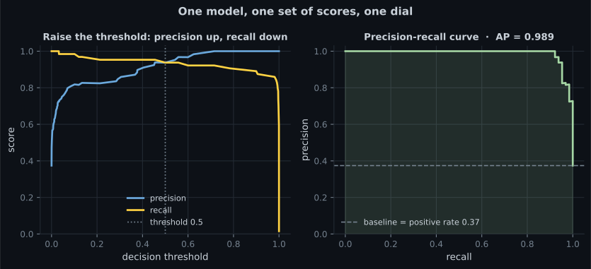
Reading the plot
Section titled “Reading the plot”| Threshold | Precision | Recall | Reading | |
|---|---|---|---|---|
| 0.1 | 0.818 | 0.984 | 0.894 | Catches 63 of 64 cancers, 14 false alarms |
| 0.3 | 0.859 | 0.953 | 0.904 | Cautious triage |
| 0.5 | 0.938 | 0.938 | 0.938 | The default |
| 0.7 | 1.000 | 0.922 | 0.959 | Best — no false alarms at all |
| 0.9 | 1.000 | 0.875 | 0.933 | Too conservative; misses 8 cases |
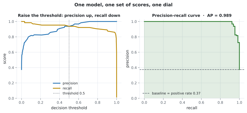
- The curves cross near 0.5, by coincidence. Nothing forces that; on imbalanced data the crossing point is usually far from the default.
- The best is at 0.7, not 0.5. A free 2-point gain, available with a one-line change.
- The PR curve’s baseline is the positive rate, here 64/171 = 0.374 — that is what a random classifier achieves, not 0.5. A PR curve hugging the top-right corner means the model is genuinely separating the classes.
Choosing a threshold deliberately
Section titled “Choosing a threshold deliberately”precision_recall_curve returns the full trade-off, so you can pick the operating point your
problem requires rather than accepting 0.5:
import numpy as np
from sklearn.datasets import load_breast_cancer
from sklearn.linear_model import LogisticRegression
from sklearn.metrics import precision_recall_curve, precision_score, recall_score
from sklearn.model_selection import train_test_split
from sklearn.pipeline import make_pipeline
from sklearn.preprocessing import StandardScaler

X, y = load_breast_cancer(return_X_y=True)
y = 1 - y
X_tr, X_te, y_tr, y_te = train_test_split(
    X, y, test_size=0.3, random_state=0, stratify=y
)

model = make_pipeline(StandardScaler(), LogisticRegression(max_iter=5000))
model.fit(X_tr, y_tr)
proba = model.predict_proba(X_te)[:, 1]

precision, recall, thresholds = precision_recall_curve(y_te, proba)

# The lowest threshold that still reaches 99% precision — lowest keeps recall high
idx = np.argmax(precision[:-1] >= 0.99)
chosen = thresholds[idx]

pred = (proba >= chosen).astype(int)
print(f"threshold  {chosen:.4f}")
print(f"precision  {precision_score(y_te, pred):.4f}")
print(f"recall     {recall_score(y_te, pred):.4f}")
The pattern generalises. For a target recall instead, scan recall >= target from the other
end. State the requirement first — “we must catch 95% of fraud” — then derive the threshold, rather
than reporting whatever 0.5 happens to give.
Average precision
Section titled “Average precision”describes a single operating point. Average precision summarises the entire curve:
the precision-weighted area under the PR curve. On the breast-cancer model, AP = 0.989, meaning precision stays near 1 across essentially the whole recall range.
| Metric | Describes | Use when |
|---|---|---|
| Precision | One operating point | False alarms are the expensive error |
| Recall | One operating point | Misses are the expensive error |
| One operating point | Both matter roughly equally | |
| One operating point | One matters times more | |
| Average precision | The whole curve | Comparing models before fixing a threshold |
| ROC-AUC | The whole curve | Classes are roughly balanced — see the next page |
Use a curve metric while choosing between models, and a point metric once you have committed to an operating point.
Pitfalls
Section titled “Pitfalls”-
Your fraud model flags 100 transactions and 30 are genuinely fraudulent, out of 50 frauds in total. What are precision and recall?
Precision = 30/100 = 0.30 (of what you flagged). Recall = 30/50 = 0.60 (of what existed). Same numerator, different denominators.
pch.quizShowAnswer
A — Precision 0.30, recall 0.60 — Precision = 30/100 = 0.30 (of what you flagged). Recall = 30/50 = 0.60 (of what existed). Same numerator, different denominators.
-
Why does F1 use a harmonic mean rather than an arithmetic one?
Precision 1.0 with recall 0.0 gives an arithmetic mean of 0.50 — misleadingly respectable. The harmonic mean gives exactly 0.
pch.quizShowAnswer
B — The harmonic mean is dominated by the smaller value, so a model cannot score well by excelling at one and failing the other — Precision 1.0 with recall 0.0 gives an arithmetic mean of 0.50 — misleadingly respectable. The harmonic mean gives exactly 0.
-
You are screening for a serious disease. Which metric should you optimise?
A missed diagnosis is far worse than a follow-up test. F2 encodes that asymmetry explicitly, rather than pretending the two errors cost the same.
pch.quizShowAnswer
B — F-beta with beta = 2, which weights recall twice as heavily as precision — A missed diagnosis is far worse than a follow-up test. F2 encodes that asymmetry explicitly, rather than pretending the two errors cost the same.
-
On a dataset with 1% positives, your model achieves average precision 0.15. Is that good?
Unlike ROC-AUC, the PR baseline moves with class balance. Always compare AP against the positive rate rather than against 0.5.
pch.quizShowAnswer
B — Yes — the random baseline for AP is the positive rate, 0.01, so this is roughly a fifteenfold improvement — Unlike ROC-AUC, the PR baseline moves with class balance. Always compare AP against the positive rate rather than against 0.5.
🧪 Try It Yourself
Section titled “🧪 Try It Yourself”Exercise 1 – Precision and recall from counts
Section titled “Exercise 1 – Precision and recall from counts”Exercise 2 – Harmonic beats arithmetic
Section titled “Exercise 2 – Harmonic beats arithmetic”Exercise 3 – Weight recall with F-beta
Section titled “Exercise 3 – Weight recall with F-beta”Exercise 4 – Find the best threshold for F1
Section titled “Exercise 4 – Find the best threshold for F1”Exercise 5 – Hit a target precision
Section titled “Exercise 5 – Hit a target precision”- Precision is “of what I flagged, how much was right”; recall is “of what existed, how much did I catch”.
- The threshold is the dial between them, and moving it needs no retraining.
- is their harmonic mean, so it is dominated by the weaker of the two: precision 1.0 with recall 0.0 gives , not 0.5.
- The ten-row example: precision 0.667, recall 0.800, 0.727, 0.769.
- encodes which error is worse; for screening, for blocking.
- Derive the threshold from a stated requirement, on validation data, and freeze it before touching the test set.
- Average precision summarises the whole curve, and its baseline is the positive rate, not 0.5.
Exercise 6 – Let each objective pick its own threshold
Section titled “Exercise 6 – Let each objective pick its own threshold”Continue to The ROC Curve and AUC — the other curve metric, what it measures that precision-recall does not, and the imbalanced case where it will flatter a model that deserves no flattery.
pch.coffeeTagline
pch.coffeeCtapch.feedbackHeading
pch.feedbackSubheading