Text Generation with Language Models

A character-level language model predicts one distribution over the next character, and generation is just sampling from it repeatedly. Every interesting decision is in how you sample, and that decision is usually explained with three printed samples and an assertion about which looks best.

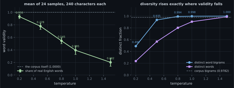
It can be measured instead. The corpus is real English, so word validity — the share of produced tokens that are dictionary words — is a quality proxy you can compute, and distinct n-grams measures diversity. Both move, in opposite directions:

Temperature	Word validity	Distinct words	Distinct bigrams	Longest repeated run
0.2	0.9301	0.2358	0.4899	5.46
0.5	0.7780	0.5675	0.9349	2.33
0.8	0.5449	0.8014	0.9942	1.71
1.0	0.3947	0.9052	0.9981	1.12
1.5	0.2021	0.9881	1.0000	1.00
the corpus itself	1.0000	0.8139	0.9782	1.46

Note the last row. Real text is not at either extreme — it sits at 0.8139 distinct words, close to temperature 0.8, while scoring validity 1.0000 that no sampling temperature reaches.

This model is small on purpose

90,643 parameters, a 40-character window, 36,000 training windows thinned evenly from the 515,595 available, 10 epochs, 372 seconds on a CPU. It produces word-shaped fragments, not sentences — the samples below are real output and they are not good. That is fine for this page: the temperature trade is visible in a weak model exactly as it is in a strong one, and pretending otherwise would require a GPU and several hours.

What you’ll learn

• What temperature does to a softmax, and the measured trade it produces.
• Why greedy decoding scored a perfect 1.0000 word validity and is still the worst setting here.
• How top-k and nucleus sampling differ from temperature, measured on the same axes.
• Why validation loss kept falling after the text stopped improving.

Temperature

Temperature divides the logits before the softmax:

$$p_i = \frac{\exp(z_i / T)}{\sum_j \exp(z_j / T)}$$

$T < 1$ sharpens the distribution towards the argmax; $T > 1$ flattens it towards uniform; $T = 1$ leaves the model’s own distribution alone. It is a single number that moves the sampler between “always the most likely character” and “ignore the model”.

Temperature, then optionally top-k or nucleus

scaled = np.log(np.clip(probabilities, 1e-12, None)) / temperature
scaled = np.exp(scaled - scaled.max())
scaled /= scaled.sum()
 
if top_k:                                  # keep the k most likely, renormalise
    keep = np.argsort(scaled)[-top_k:]
    mask = np.zeros_like(scaled); mask[keep] = scaled[keep]
    scaled = mask / mask.sum()
 
if top_p:                                  # keep the smallest set summing to p
    order = np.argsort(scaled)[::-1]
    cut = int(np.searchsorted(np.cumsum(scaled[order]), top_p)) + 1
    mask = np.zeros_like(scaled); mask[order[:cut]] = scaled[order[:cut]]
    scaled = mask / mask.sum()

The + 1 in the nucleus cut is not a rounding detail — without it, a step where one character already exceeds $p$ would keep nothing at all.

figure 24 samples of 240 characters at each setting matplotlib

The two panels are mirror images, which is the whole point: there is no temperature that is best on both axes. The corpus reference lines matter more than the curves — real text scores 1.0000 validity and 0.9782 distinct bigrams simultaneously, and no sampling temperature gets close to both, because the model is not good enough. Temperature cannot fix a weak model, only choose which way it fails.

Greedy decoding scores perfectly and is useless

Setting temperature to zero — always take the most likely character — produced this:

greedy, 220 characters

the the the the the the the the the the the the the the the the the the the the the the the
the the the the the the the the the the the the the the the the the the the the the the the

Its measured scores:

Strategy	Word validity	Distinct words	Distinct bigrams	Longest repeated run
greedy	1.0000	0.0171	0.0174	58.33
T = 0.5	0.7780	0.5675	0.9349	2.33
T = 1.0	0.3947	0.9052	0.9981	1.12
top-k = 5, T = 1.0	0.6619	0.6894	0.9868	1.62
nucleus p = 0.9, T = 1.0	0.4912	0.8255	0.9966	1.17

Word validity 1.0000 — a perfect score. the is a dictionary word, so a model that writes nothing else is, by that metric alone, flawless. The longest-repeat column is what exposes it: 58.33 consecutive repetitions against 1.46 for real English.

This is the same failure the evaluation page found when 200 copied images beat real data on the Fréchet distance. A single generative metric is not a score to maximise — it is one of several constraints, and the degenerate solution usually maxes exactly one of them.

figure Same model, same number of characters, five decoding rules matplotlib

Greedy is off the scale on the right panel and perfect on the left — the clearest demonstration in this phase that a metric with a degenerate optimum will find it. Among the real strategies, top-k = 5 lands closest to the corpus on both axes: validity 0.6619 with 0.9868 distinct bigrams, against the corpus's 1.0000 and 0.9782.

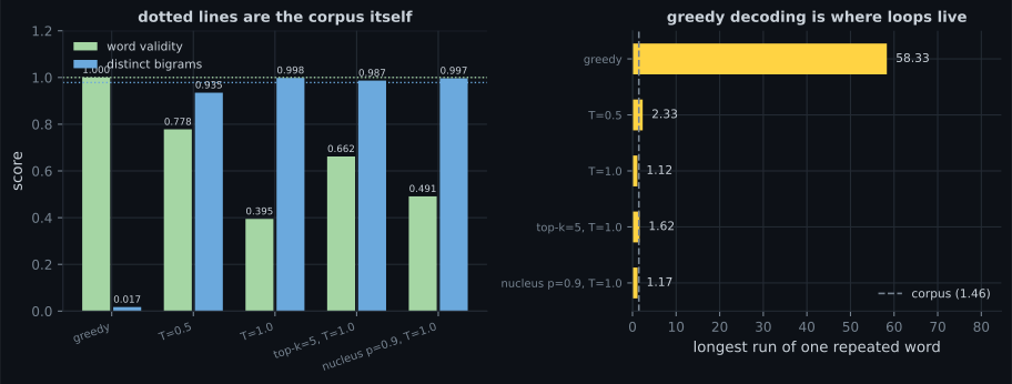
Top-k and nucleus sampling both attack the same problem from a different direction than temperature. Temperature reweights every character, including ones the model considers absurd; top-k and nucleus delete the tail first and then sample normally from what remains. That is why top-k = 5 at T = 1.0 (validity 0.6619) beats plain T = 1.0 (0.3947) while keeping almost all its diversity — 0.9868 distinct bigrams against 0.9981.

diagram Diagram mermaid

  flowchart LR
  L["logits"] --> T["divide by temperature"]
  T --> S["softmax"]
  S --> K{"truncate?"}
  K -->|"top-k: keep k best"| R["renormalise"]
  K -->|"nucleus: keep smallest set summing to p"| R
  K -->|"neither"| D["sample"]
  R --> D
  D -.->|"T low: validity 0.9301, repeats 5.46"| A["safe and dull"]
  D -.->|"T high: validity 0.2021, repeats 1.00"| B["varied and wrong"]
  D -.->|"top-k 5: 0.6619 / 0.9868"| C["closest to the corpus"]

sketch Temperature, top-k and nucleus on one distribution p5.js Pause Restart

Drag the temperature slider and click a truncation rule. The bars are the resulting sampling distribution, with the measured validity and diversity for that temperature.

Loss keeps falling after the text stops improving

figure 10 epochs, 90,643 parameters, 372s matplotlib

The left panel is the smooth curve everyone reports. The right one is what it buys, and it is far noisier — validity moves 0.7222, 0.7778, 0.8333, 0.7838 across consecutive epochs while the loss falls monotonically. A single sample scored at one checkpoint is a noisy measurement, which is why the temperature table above averages 24 samples per setting.

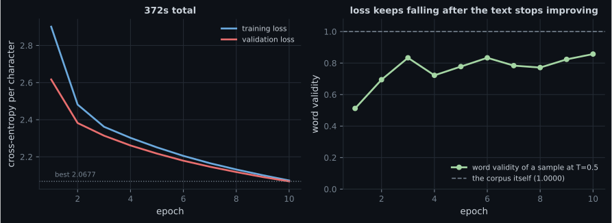
Epoch	Loss	Validation loss	Sample validity
1	2.9012	2.6169	0.5122
3	2.3618	2.3139	0.8333
6	2.2051	2.1791	0.8333
10	2.0727	2.0677	0.8571

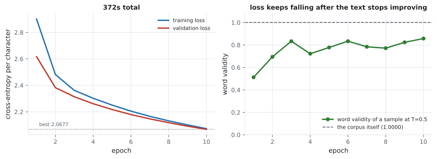
Cross-entropy per character fell 2.9012 → 2.0727 with no sign of overfitting — validation tracks training within 0.005 at the end, which says the model is under-fitting and would benefit from more capacity and more data rather than from regularisation.

What the samples look like at each stage is the more honest progress report:

epoch 1, T=0.5

o te te are te aie te wte hes aor t rh toie thh tlo ta tot f tos aort so t torn eo t taihe

epoch 10, T=0.5

 at rore the fill br how of the the macter the br the br the of of the the prove the the reack

By epoch 10 the model has learned English letter statistics and a handful of very common words (the, of, and, in), and nothing about meaning. br appears constantly because the corpus is IMDB reviews decoded from token ids, where br — from the HTML line breaks in the original reviews — survived tokenisation as a frequent word.

sketch The measured table, ranked p5.js Pause Restart

Click a column to rank every row by it. The bars are that column's values and the highest and lowest are computed from the numbers, not written in.

Pitfalls

• Reporting one sample per temperature. Validity varies by ±0.03 to ±0.07 across samples at a fixed setting; the tables here average 24.
• Maximising a single text metric. Greedy decoding scored 1.0000 word validity by repeating one word 58 times.
• Reading validation loss as sample quality. Loss fell monotonically while sample validity moved 0.7222 → 0.7778 → 0.8333 → 0.7838 between consecutive epochs.
• Confusing temperature with truncation. Temperature reweights the whole distribution; top-k and nucleus delete the tail. Top-k = 5 at T = 1.0 scored 0.6619 against plain T = 1.0’s 0.3947, at almost the same diversity.
• Forgetting the + 1 in the nucleus cut. A step where one character already exceeds p would otherwise keep no characters at all.
• Generating one sample at a time. A forward pass costs the same for 1 row as for 24, so batch the samples — generating them serially multiplies the wall-clock for nothing.
• Expecting sentences from a character model this size. 90,643 parameters and ten epochs buy letter statistics and common short words.

Recap

• Temperature divides the logits before the softmax, trading validity against diversity: 0.9301 validity at T = 0.2 down to 0.2021 at T = 1.5, with distinct words moving 0.2358 → 0.9881 the other way.
• The corpus itself scores 1.0000 validity and 0.9782 distinct bigrams — no temperature setting reaches both, because temperature cannot repair a weak model.
• Greedy decoding is the degenerate optimum of word validity: a perfect 1.0000, with a 58.33-token repeated run.
• Truncation beats reweighting here: top-k = 5 at T = 1.0 gave 0.6619 validity with 0.9868 distinct bigrams.
• Loss and sample quality decouple — validation loss fell smoothly while validity bounced.
• Always average several samples per setting, and always report a corpus baseline.

Next

Two techniques that generate without a generator at all — freeze a trained network and optimise the input instead: DeepDream.

pch.quizTag pch.quizDefaultTitle

1. Greedy decoding scored a perfect 1.0000 word validity. Why is it still the worst strategy measured here?

   A Because greedy decoding is slower B Because it produced one word repeated 58 times — 'the' is a dictionary word, so a degenerate output maximises that single metric while scoring 0.0171 on distinct words C Because validity is measured incorrectly D Because it needs a higher temperature to work
   pch.quizShowAnswer

   B — Because it produced one word repeated 58 times — 'the' is a dictionary word, so a degenerate output maximises that single metric while scoring 0.0171 on distinct words — This is the same shape of failure as copied images beating real data on FID: any single generative metric has a degenerate optimum, so you need at least two that pull in opposite directions.

2. What does raising the sampling temperature do to the softmax?

   A It removes unlikely characters from consideration B It divides the logits before the softmax, flattening the distribution towards uniform — which raised distinct words from 0.2358 to 0.9881 and dropped validity from 0.9301 to 0.2021 C It increases the model's confidence D It changes the model's weights
   pch.quizShowAnswer

   B — It divides the logits before the softmax, flattening the distribution towards uniform — which raised distinct words from 0.2358 to 0.9881 and dropped validity from 0.9301 to 0.2021 — Temperature reweights every character including the implausible ones, which is exactly why very high temperatures produce diverse nonsense.

3. How does top-k sampling differ from simply lowering the temperature?

   A It is mathematically identical B It deletes the unlikely tail entirely and then samples normally, rather than reweighting everything — which gave 0.6619 validity at T=1.0 against 0.3947 for plain T=1.0, at nearly the same diversity C It always produces the most likely token D It only applies to word-level models
   pch.quizShowAnswer

   B — It deletes the unlikely tail entirely and then samples normally, rather than reweighting everything — which gave 0.6619 validity at T=1.0 against 0.3947 for plain T=1.0, at nearly the same diversity — Truncation removes the characters the model considers absurd while leaving the relative probabilities of the plausible ones untouched.

4. Validation loss fell smoothly from 2.6169 to 2.0677 while sample validity moved 0.7222, 0.7778, 0.8333, 0.7838 across consecutive epochs. What follows?

   A The validity measurement is broken B Loss and sample quality are only loosely coupled, and a single sample per checkpoint is a noisy measurement — which is why the temperature results average 24 samples per setting C The model is overfitting D The learning rate is too high
   pch.quizShowAnswer

   B — Loss and sample quality are only loosely coupled, and a single sample per checkpoint is a noisy measurement — which is why the temperature results average 24 samples per setting — Validation loss also tracked training loss to within 0.005, which indicates under-fitting rather than overfitting.

5. The corpus itself scored validity 1.0000 and distinct bigrams 0.9782, while no temperature achieved both. What does that tell you?

   A The metrics are on incomparable scales B Temperature only chooses how a weak model fails — it cannot move the model onto the corpus's operating point, which would require a better model C The corpus baseline is computed wrongly D A temperature between 0.8 and 1.0 does achieve both
   pch.quizShowAnswer

   B — Temperature only chooses how a weak model fails — it cannot move the model onto the corpus's operating point, which would require a better model — That is why reporting a corpus baseline matters: without it, temperature 0.2's 0.9301 validity looks like near-perfect text rather than repetitive fragments.

🧪 Try It Yourself

pch.exerciseTag pch.exerciseTitle

pch.exerciseTag pch.exerciseTitle

pch.exerciseTag pch.exerciseTitle

pch.exerciseTag pch.exerciseTitle

pch.exerciseTag pch.exerciseTitle

pch.exerciseTag pch.exerciseTitle