Vanishing & Exploding Gradients

Backpropagation multiplies. Every layer’s gradient is the product of the terms above it, and a product of twenty numbers has only two interesting behaviours: it collapses toward zero or it runs away. Both are measured below, along with the three fixes — activation choice, initialisation, and clipping — that made depth trainable in the first place.

What you’ll learn

• The measured gradient norm reaching layer 1 of a 20-layer sigmoid network: 1.19e−12, against 0.67 with ReLU and He.
• Why that number is no accident: $0.25^{20} =$ 9.09e−13, sigmoid’s analytic best case.
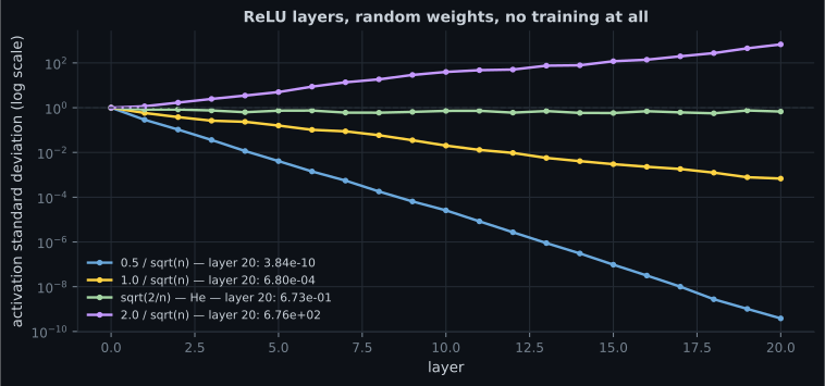
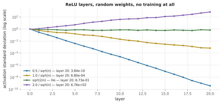
• How initialisation scale decides whether the forward signal survives — measured from 3.84e−10 to 6.76e+02 across four scales.
• Why He uses $\sqrt{2/n}$ where Glorot uses $\sqrt{1/n}$.
• An exploding run that reached a first-epoch loss of 25,528 and killed 127 of 128 ReLU units.
• clipnorm against clipvalue, and why one preserves the update direction and the other does not.

The problem is a product

For a network of $L$ layers, the gradient reaching layer $\ell$ is

$$\frac{\partial L}{\partial \mathbf{W}_\ell} = \frac{\partial L}{\partial \mathbf{a}_L} \left( \prod_{k=\ell+1}^{L} \frac{\partial \mathbf{a}_k}{\partial \mathbf{a}_{k-1}} \right) \frac{\partial \mathbf{a}_\ell}{\partial \mathbf{W}_\ell}$$

Each factor is a weight matrix times an activation derivative. If the typical factor has magnitude 0.8, then after 20 layers you have $0.8^{20} = 0.012$; at 0.5 you have $9.5 \times 10^{-7}$; at 1.2 you have 38. There is no stable middle unless something forces the factors close to 1.

figure One backward pass through 20 hidden layers matplotlib

Layer 1 is nearest the input, layer 20 nearest the output. With sigmoid and Glorot the gradient shrinks by a factor of 4.07e-12 on its way to the first layer, which in float32 is indistinguishable from no update at all. tanh and ReLU+He both stay inside a factor of 4.2 across the entire depth — flat enough that every layer learns.

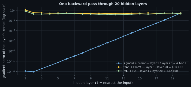
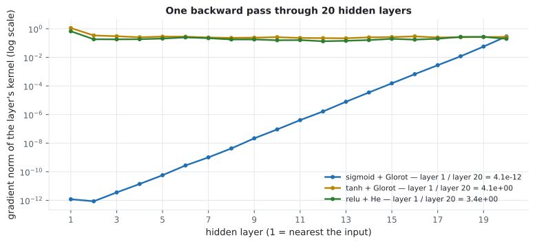
Configuration	Layer 1 gradient norm	Layer 20	Ratio
sigmoid + Glorot	1.1885e−12	2.9207e−01	4.0691e−12
tanh + Glorot	1.1224e+00	2.7119e−01	4.1388e+00
relu + He	6.6840e−01	1.9814e−01	3.3733e+00

The first row is the vanishing gradient, measured. The first layer of that network receives an update roughly a trillion times smaller than the last layer’s — so training reports a falling loss while the early layers stay frozen at their random initialisation.

Why sigmoid, specifically

$$\sigma'(z) = \sigma(z)\big(1 - \sigma(z)\big) \qquad \max_z \sigma'(z) = \sigma'(0) = 0.25$$

$z$	$\sigma(z)$	$\sigma'(z)$
0.0	0.500000	0.250000
±2.0	0.880797	0.104994
±4.0	0.982014	0.017663
±6.0	0.997527	0.002467

The derivative’s maximum is 0.25, so even in the best possible case every layer divides the gradient by at least four:

Depth	Best case $0.25^{\text{depth}}$
5	9.7656e−04
10	9.5367e−07
20	9.0949e−13
50	7.8886e−31

Compare $0.25^{20} = 9.09 \times 10^{-13}$ with the measured 20-layer value of $1.19 \times 10^{-12}$. The measurement lands within a factor of 1.3 of the theoretical ceiling — the network is operating at sigmoid’s best case and still failing, which makes this a property of the activation rather than a tuning problem. ReLU’s derivative is exactly 1 wherever the unit is active, so the product does not shrink at all; tanh’s peaks at 1.0 rather than 0.25, which is why it was the pre-ReLU default.

diagram Diagram mermaid

  flowchart TD
  A["gradients die or explode
with depth"] --> B{"activation derivative
peaks below 1?"}
  B -- "sigmoid: 0.25" --> C["use relu (1.0)
or tanh (1.0)"]
  A --> D{"weights scaled wrong
for the fan-in?"}
  D -- yes --> E["he_normal for relu
glorot for tanh and sigmoid"]
  A --> F{"still exploding
on some batches?"}
  F -- yes --> G["clipnorm on the optimizer"]
  C --> H["deep network trains"]
  E --> H
  G --> H
  I["or normalise activations
at every layer"] --> H

Initialisation: keeping the variance at 1

Push a signal with unit variance through a layer of $n$ inputs whose weights have standard deviation $s$. Each output is a sum of $n$ independent products, so its variance is $n s^2$. To keep variance at 1 you need $s = 1/\sqrt{n}$ — that is Glorot (Xavier), give or take the fan-out averaging.

ReLU then zeroes half the outputs, halving the variance again. Compensate with a factor of 2 inside the square root:

$$s_{\text{Glorot}} = \sqrt{\frac{1}{n_{\text{in}}}} \qquad s_{\text{He}} = \sqrt{\frac{2}{n_{\text{in}}}}$$

Measured with random weights and no training at all — 512 samples pushed through 20 ReLU layers of 60 units:

figure ReLU layers, random weights, no training at all matplotlib

The dashed line marks a standard deviation of 1. Only the He scale, sqrt(2/n), holds the signal steady across twenty layers — it ends at 0.673. Scale 1.0, which is Glorot's value and correct for tanh, decays to 6.8e-04 because ReLU keeps halving the variance. Scale 2.0 amplifies instead and ends 675 times too large.

Weight scale	Layer 0	Layer 5	Layer 20
$0.5/\sqrt{n}$	0.9979	4.0985e−03	3.8388e−10
$1.0/\sqrt{n}$ (Glorot)	0.9979	1.5895e−01	6.7952e−04
$\sqrt{2/n}$ (He)	0.9979	7.3706e−01	6.7263e−01
$2.0/\sqrt{n}$	0.9979	5.0020e+00	6.7552e+02

No gradients are involved here — this is the forward pass. A signal that has decayed to 1e-10 by layer 20 carries no information for the backward pass to work with, which is why initialisation matters before any optimiser is chosen.

Two lines that decide whether a deep network trains

keras.layers.Dense(64, activation="relu", kernel_initializer="he_normal")
keras.layers.Dense(64, activation="tanh", kernel_initializer="glorot_uniform")

Keras defaults to glorot_uniform for every layer, so a deep ReLU network on defaults is using the wrong initialiser. It usually still trains — the Glorot row above lands at 6.8e-04 rather than zero — but it starts from a worse place for no reason.

sketch Push a signal through 20 layers p5.js Pause Restart

Real random matrices, recomputed on demand: drag the weight scale and watch the activation spread across twenty ReLU layers collapse, hold, or explode.

Non-saturating activations

Activation	Derivative range	Saturates?
sigmoid	(0, 0.25]	in both directions
tanh	(0, 1]	in both directions
ReLU	$\{0, 1\}$	for negatives, permanently
Leaky ReLU (α=0.01)	$\{0.01, 1\}$	no
ELU / SELU	(0, 1]	no

ReLU’s failure mode differs in kind: it does not squash the gradient, it switches it off entirely for any unit whose pre-activation has gone negative everywhere. That unit’s gradient is exactly zero, so it can never recover — measured below. Leaky ReLU exists to leave a 0.01 slope so recovery stays possible. The full activation comparison, including the run where tanh beat ReLU at depth 8, is on the activation functions page.

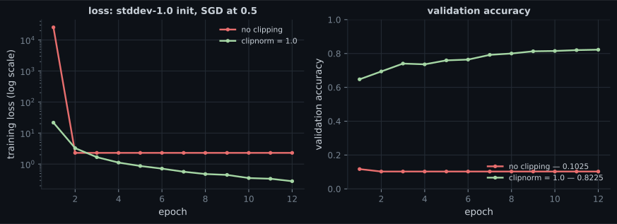
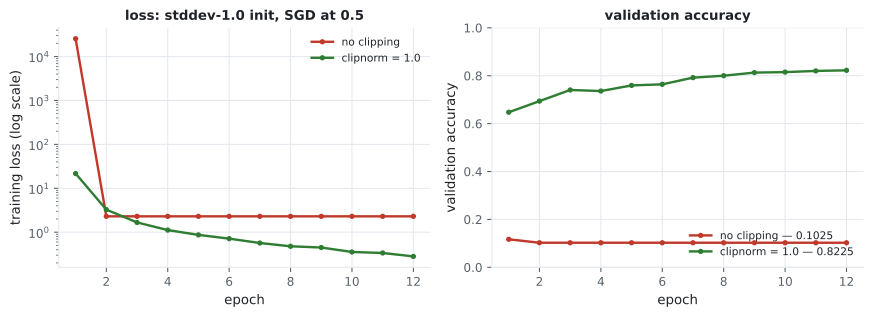
Exploding gradients, and clipping

Take a shallow network, initialise the weights with standard deviation 1.0 — roughly 30× too large for a 784-input layer — and use SGD at 0.5:

figure The same initialisation, with and without clipnorm matplotlib

The unclipped run's first-epoch loss is 25,528. It then flatlines at 2.3012 — which is ln(10) = 2.3026, exactly the loss of predicting a uniform distribution over ten classes. The network has not stalled; it has died. clipnorm=1.0 turns the identical setup into a normal run ending at 0.8225 accuracy.

	Epoch 1 loss	Final loss	Final val accuracy
no clipping	25,528.77	2.3012	0.1025
clipnorm=1.0	21.66	0.2812	0.8225

The flatline at 2.30 is diagnostic. $\ln(10) = 2.3026$ is the cross-entropy of a model outputting a uniform distribution over ten classes — the loss of a network that has stopped saying anything. Counting the units confirms it:

	Dead units in layer 1	Mean activation
no clipping	127 of 128	0.0000
clipnorm=1.0	0 of 128	2.7444

One enormous first update drove 127 of 128 ReLU units permanently negative. Their gradients are zero, so they never came back. The loss curve looked like a plateau; the network was a corpse. Any time a classification loss sits at $\ln(\text{classes})$, check for dead units before touching the learning rate.

clipnorm against clipvalue

Two different operations

keras.optimizers.SGD(0.5, clipnorm=1.0)    # rescale the whole gradient vector
keras.optimizers.SGD(0.5, clipvalue=1.0)   # truncate each component separately

For a gradient of [3.0, 4.0, 0.5] with norm 5.0249:

	Result	Norm	Direction
clipnorm=1.0	[0.5970, 0.7960, 0.0995]	1.0000	preserved
clipvalue=1.0	[1.0000, 1.0000, 0.5000]	1.5000	changed (cosine 0.9619)

clipnorm scales the vector, so the update still points down the steepest-descent direction — just less far. clipvalue truncates each component independently, which changes where the step goes; here the cosine with the true gradient drops to 0.9619. Prefer clipnorm unless you specifically need per-component bounds.

sketch The measured table, ranked p5.js Pause Restart

Click a column to rank every row by it. The bars are that column's values and the highest and lowest are computed from the numbers, not written in.

Pitfalls

• Leaving the default initialiser on a deep ReLU network. Keras defaults to glorot_uniform everywhere; ReLU wants he_normal.
• Reading a flat loss as “needs more epochs”. At $\ln(\text{classes})$ the model is uniform. Check for dead units.
• Using sigmoid in hidden layers. Its derivative caps at 0.25, so 20 layers cost a factor of at least $4^{20}$.
• Assuming vanishing gradients show up in the loss. They do not: the last layers keep learning and the loss keeps falling while the first layers stay frozen. Print per-layer gradient norms.
• Using clipvalue when you meant clipnorm. One preserves the descent direction; the other does not.
• Clipping as a first resort. It masks exploding gradients; a wrong initialiser or too high a learning rate is usually the real cause.
• Forgetting that a dead ReLU is permanent. Leaky ReLU, ELU or a lower learning rate prevent it; nothing repairs one afterwards.

Recap

• Every layer’s gradient is a product of the layers above it, so depth either collapses or amplifies unless the typical factor sits near 1.
• Measured over 20 layers: sigmoid delivered 1.19e−12 to layer 1, a ratio of 4.07e−12 against the last layer; tanh and ReLU+He stayed within a factor of 4.2.
• Sigmoid’s derivative caps at 0.25, giving a best case of 9.09e−13 over 20 layers — and the measurement matched that ceiling within a factor of 1.3.
• Keeping forward variance at 1 needs $s = \sqrt{1/n}$ (Glorot); ReLU’s halving needs $\sqrt{2/n}$ (He). Only He held the spread flat, at 0.673 after 20 layers.
• An over-large initialisation with SGD at 0.5 gave a first-epoch loss of 25,528, killed 127 of 128 units, and flatlined at ln(10).
• clipnorm rescales the gradient and preserves direction; clipvalue truncates components and does not.

Next

Initialisation fixes the starting variance. Nothing keeps it fixed once the weights begin moving — which is what normalisation layers are for: Batch Normalization.

pch.quizTag pch.quizDefaultTitle

1. A 20-layer sigmoid network shows a layer-1 gradient norm of 1.19e-12 while its layer-20 norm is 0.29. What will the training curve look like?

   A The loss will not move at all B The loss will fall normally, because the layers near the output are still learning — the early layers are frozen at their random initialisation and nothing in the loss curve reveals it C The loss will oscillate wildly D Training will crash with a numerical error
   pch.quizShowAnswer

   B — The loss will fall normally, because the layers near the output are still learning — the early layers are frozen at their random initialisation and nothing in the loss curve reveals it — This is why vanishing gradients are dangerous: the symptom is invisible in the metric you watch. Print per-layer gradient norms.

2. Why does He initialisation use sqrt(2/n) where Glorot uses sqrt(1/n)?

   A Because ReLU networks are usually deeper B Because ReLU zeroes roughly half its outputs, halving the variance at every layer — the factor of 2 inside the root compensates for exactly that loss C Because He was designed for convolutional layers D Because larger weights train faster
   pch.quizShowAnswer

   B — Because ReLU zeroes roughly half its outputs, halving the variance at every layer — the factor of 2 inside the root compensates for exactly that loss — Measured over 20 ReLU layers: scale 1.0/sqrt(n) decayed to 6.8e-04 while sqrt(2/n) held at 0.673.

3. A ten-class classifier's loss sits at exactly 2.30 and never moves. What should you check first?

   A Whether the learning rate is too low B Whether the ReLU units are dead — ln(10) = 2.3026 is the loss of a uniform prediction, and one oversized update can drive nearly every unit permanently negative C Whether the dataset is shuffled D Whether the batch size is too large
   pch.quizShowAnswer

   B — Whether the ReLU units are dead — ln(10) = 2.3026 is the loss of a uniform prediction, and one oversized update can drive nearly every unit permanently negative — In the measured run, 127 of 128 layer-1 units output zero for every input. Their gradients are zero, so further training cannot recover them.

4. What is the difference between clipnorm=1.0 and clipvalue=1.0 for a gradient of [3.0, 4.0, 0.5]?

   A They produce the same result B clipnorm scales the whole vector to norm 1.0 and preserves its direction; clipvalue truncates each component into [-1, 1], giving [1.0, 1.0, 0.5] with norm 1.5 and a different direction C clipvalue is always safer because it bounds each component D clipnorm only applies to recurrent layers
   pch.quizShowAnswer

   B — clipnorm scales the whole vector to norm 1.0 and preserves its direction; clipvalue truncates each component into [-1, 1], giving [1.0, 1.0, 0.5] with norm 1.5 and a different direction — The clipvalue result has cosine 0.9619 with the true gradient — it no longer points down the steepest-descent direction.

5. Sigmoid's derivative peaks at 0.25, so 20 layers give a best case of 9.09e-13. The measured layer-1 gradient was 1.19e-12. What does that agreement tell you?

   A The measurement must be wrong, since it exceeds the bound B The network is operating essentially at sigmoid's theoretical best case and still failing, so this is a structural property of the activation rather than a tuning problem C The bound only applies beyond 50 layers D The weights must have been initialised badly
   pch.quizShowAnswer

   B — The network is operating essentially at sigmoid's theoretical best case and still failing, so this is a structural property of the activation rather than a tuning problem — Within a factor of 1.3 of the ceiling. No learning rate, optimiser or schedule fixes a factor of 4 lost per layer — the activation has to change.

🧪 Try It Yourself

pch.exerciseTag pch.exerciseTitle

pch.exerciseTag pch.exerciseTitle

pch.exerciseTag pch.exerciseTitle

pch.exerciseTag pch.exerciseTitle

pch.exerciseTag pch.exerciseTitle

pch.exerciseTag pch.exerciseTitle