What you’ll learn

• what changes when the target becomes a label instead of a number
• the decision boundary, and why each algorithm can only draw certain shapes
• why every good classifier outputs a probability, and the threshold turns it into a label
• the accuracy paradox: 98% accuracy from a model that never predicts the positive class
• binary, multiclass, multilabel and multioutput — four problems that get confused
• the ten-row example this whole phase reuses

Intuition

Regression asks how much. Classification asks which one. That sounds like a small change and is not, because closeness stops counting. Predicting 302 when the truth is 300 is nearly right; predicting “benign” when the truth is “malignant” is simply wrong, and how confident the model was does not change the outcome for the patient.

Two consequences follow immediately, and they shape everything in this phase:

1. Squared error is the wrong loss. The distance between “cat” and “dog” is not a number. Classification uses log loss, hinge loss, or impurity instead.
2. Accuracy is the wrong metric more often than you would guess. It weighs every error the same, and almost no real problem does.

  flowchart LR
  X["Features x"] --> M["Model"]
  M --> S["Score  s(x)"]
  S --> P["Probability  p = sigma(s)"]
  P --> T{"p ≥ threshold?"}
  T -->|yes| POS["predict positive"]
  T -->|no| NEG["predict negative"]

Note where the threshold sits: outside the model. Training produces the probability; the threshold is a business decision you make afterwards, and changing it changes every metric without retraining anything.

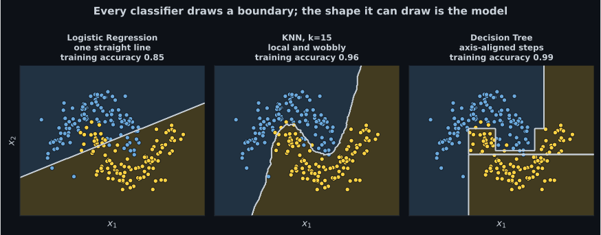
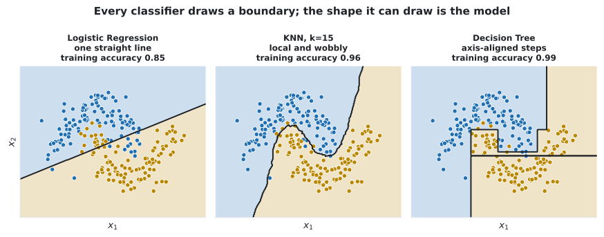
Decision boundaries

A classifier partitions the feature space into regions, one per class. The surface between regions is the decision boundary, and the shapes a model can draw are exactly its capacity.

figureThree classifiers, one datasetmatplotlib

Reading the plot

• Logistic regression manages 0.85 on this data and cannot do better, because no single straight line separates two interleaved crescents. That is a bias limitation, not a tuning problem.
• KNN traces the actual shape and reaches 0.96 — but look at the small islands near the boundary, each one caused by a handful of points.
• The tree scores 0.99 with a completely different geometry: every edge is parallel to an axis, because every split is a threshold on one feature. That near-perfect training score should also make you suspicious, and Decision Trees explains why.

None of these is “the best classifier”. They are three different assumptions about what a boundary is allowed to look like.

The accuracy paradox

figure98% accurate, and completely uselessmatplotlib

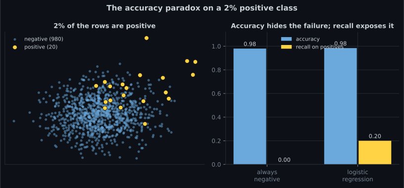
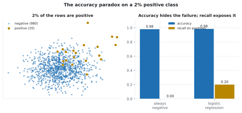
This is not a contrived example; it is fraud detection, disease screening, defect inspection, and churn prediction. Whenever the interesting class is rare, accuracy is dominated by the boring class and stops carrying information.

import numpy as np
from sklearn.dummy import DummyClassifier
from sklearn.linear_model import LogisticRegression
from sklearn.metrics import accuracy_score, recall_score
 
rng = np.random.default_rng(7)
n, positive_rate = 1000, 0.02
n_pos = int(n * positive_rate)
 
X = np.vstack([rng.normal(0, 1, (n - n_pos, 2)), rng.normal(1.6, 1.1, (n_pos, 2))])
y = np.r_[np.zeros(n - n_pos, dtype=int), np.ones(n_pos, dtype=int)]
 
for name, model in [
    ("always negative", DummyClassifier(strategy="most_frequent")),
    ("logistic regression", LogisticRegression()),
]:
    model.fit(X, y)
    pred = model.predict(X)
    print(f"{name:<20} accuracy {accuracy_score(y, pred):.4f}"
          f"   recall {recall_score(y, pred, zero_division=0):.4f}")
 
# always negative      accuracy 0.9800   recall 0.0000
# logistic regression  accuracy 0.9840   recall 0.2000

import numpy as np
from sklearn.dummy import DummyClassifier
from sklearn.linear_model import LogisticRegression
from sklearn.metrics import accuracy_score, recall_score
 
rng = np.random.default_rng(7)
n, positive_rate = 1000, 0.02
n_pos = int(n * positive_rate)
 
X = np.vstack([rng.normal(0, 1, (n - n_pos, 2)), rng.normal(1.6, 1.1, (n_pos, 2))])
y = np.r_[np.zeros(n - n_pos, dtype=int), np.ones(n_pos, dtype=int)]
 
for name, model in [
    ("always negative", DummyClassifier(strategy="most_frequent")),
    ("logistic regression", LogisticRegression()),
]:
    model.fit(X, y)
    pred = model.predict(X)
    print(f"{name:<20} accuracy {accuracy_score(y, pred):.4f}"
          f"   recall {recall_score(y, pred, zero_division=0):.4f}")
 
# always negative      accuracy 0.9800   recall 0.0000
# logistic regression  accuracy 0.9840   recall 0.2000

Always compute the DummyClassifierDummyClassifier score first. If your model’s accuracy is close to it, the accuracy number is telling you about the class balance, not about your model.

See it move

The sketch sweeps the positive rate from 50% down to 0.5% and reports two models on 1,000 rows: a DummyClassifierDummyClassifier that always says negative, and a detector that catches 20% of positives with a 1% false-positive rate. Watch which metrics notice the difference between them.

The accuracy row is the one to watch, and it does something worse than going flat:

Once positives are rare, the detector’s ten false positives cost more accuracy than its one true positive earns, so accuracy ranks the model that finds nothing above the model that finds something. Recall reads 0.0000 against 0.2000 at every row of that table — exactly as distinguishable at 0.5% as at 50%. Rarity does not make the models more similar; it makes accuracy stop measuring them, and then quietly reverses the ranking.

The ten-row example

Phase 4 reuses one small prediction set across all four evaluation pages, so the arithmetic stays comparable. Ten emails, ranked by the model’s estimated probability of being spam:

Counting the outcomes gives TP = 4, FP = 2, FN = 1, TN = 3, and from those five numbers every metric in this phase follows:

Three different numbers describing one set of predictions. Reporting only the first would be technically true and practically misleading.

Four kinds of classification problem

The distinction that trips people up is multiclass versus multilabel. Multiclass classes are mutually exclusive — a digit cannot be both a 3 and a 7. Multilabel classes are not — a photo can contain a dog and a beach. Softmax is for the first; independent sigmoids are for the second, and using softmax on a multilabel problem quietly forces the labels to compete.

A first classifier, end to end

from sklearn.datasets import load_breast_cancer
from sklearn.dummy import DummyClassifier
from sklearn.linear_model import LogisticRegression
from sklearn.model_selection import train_test_split
from sklearn.pipeline import make_pipeline
from sklearn.preprocessing import StandardScaler
 
X, y = load_breast_cancer(return_X_y=True)
y = 1 - y                      # flip so 1 = malignant, the class we want to catch
 
X_train, X_test, y_train, y_test = train_test_split(
    X, y, test_size=0.3, random_state=0, stratify=y      # stratify keeps the ratio
)
 
baseline = DummyClassifier(strategy="most_frequent").fit(X_train, y_train)
model = make_pipeline(
    StandardScaler(), LogisticRegression(max_iter=5000)
).fit(X_train, y_train)
 
print(f"baseline accuracy = {baseline.score(X_test, y_test):.4f}")  # 0.6257
print(f"model accuracy    = {model.score(X_test, y_test):.4f}")     # 0.9532
 
proba = model.predict_proba(X_test)[:, 1]
print(f"first five probabilities: {proba[:5].round(3)}")

from sklearn.datasets import load_breast_cancer
from sklearn.dummy import DummyClassifier
from sklearn.linear_model import LogisticRegression
from sklearn.model_selection import train_test_split
from sklearn.pipeline import make_pipeline
from sklearn.preprocessing import StandardScaler
 
X, y = load_breast_cancer(return_X_y=True)
y = 1 - y                      # flip so 1 = malignant, the class we want to catch
 
X_train, X_test, y_train, y_test = train_test_split(
    X, y, test_size=0.3, random_state=0, stratify=y      # stratify keeps the ratio
)
 
baseline = DummyClassifier(strategy="most_frequent").fit(X_train, y_train)
model = make_pipeline(
    StandardScaler(), LogisticRegression(max_iter=5000)
).fit(X_train, y_train)
 
print(f"baseline accuracy = {baseline.score(X_test, y_test):.4f}")  # 0.6257
print(f"model accuracy    = {model.score(X_test, y_test):.4f}")     # 0.9532
 
proba = model.predict_proba(X_test)[:, 1]
print(f"first five probabilities: {proba[:5].round(3)}")

Two details that matter more than they look:

• stratify=ystratify=y keeps the class ratio identical in both splits. Without it, a random split of an imbalanced dataset can put almost every positive case on one side.
• predict_probapredict_proba is the real output. predictpredict is just predict_proba() >= 0.5predict_proba() >= 0.5, and that 0.5 is a default nobody chose for your problem.

Pitfalls

🧪 Try It Yourself

Exercise 1 – Build a binary target

Exercise 2 – Count the four outcomes by hand

Exercise 3 – Beat the dummy baseline

Exercise 4 – Probabilities, not labels

Exercise 5 – Watch the accuracy paradox appear

Recap

• Classification predicts a label; closeness stops counting, so squared error is replaced by log loss, hinge loss or impurity.
• The decision boundary is the model’s signature — straight for logistic regression, local for KNN, axis-aligned steps for a tree.
• Models produce probabilities. predict()predict() applies a threshold of 0.5, and that threshold is yours to change.
• With a 2% positive rate, “always negative” scores 0.98 accuracy and 0.00 recall. Always compare against DummyClassifierDummyClassifier.
• The ten-row example gives TP = 4, FP = 2, FN = 1, TN = 3 — accuracy 0.70, precision 0.667, recall 0.80.
• Multiclass labels are mutually exclusive; multilabel ones are not.

Exercise 6 – Find the prevalence where accuracy inverts

Next

Continue to Logistic Regression (Binary vs Multiclass) — the classifier that produces those probabilities, derived from the linear model of Phase 3.