Word Embeddings (Word2Vec, GloVe)

A bag of words gives every word its own column, so good and great are as unrelated as good and refrigerator. An embedding replaces that with a dense vector per word, learned so that words used similarly end up close together.

The word “similarly” is doing a lot of work in that sentence, and this page is mostly about it. The same corpus, trained two ways, produces two different notions of similarity — and one of them collapses onto a single dimension.

What you’ll learn

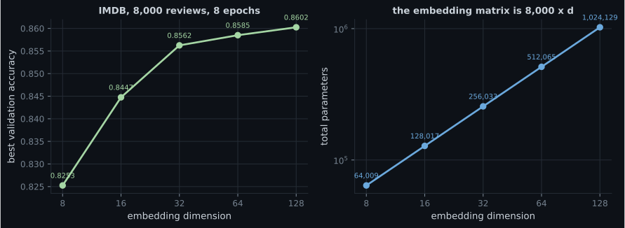
• Why an embedding is a lookup table, and how its size scales: 8 dimensions is 64,000 parameters, 128 is 1,024,000.
• What accuracy the extra width actually buys: +0.0350 for 16× the embedding matrix.
• The measured difference between embeddings trained on a label and on co-occurrence.
• Why sentiment-trained vectors reach cosine similarity 1.000 — and why that is a failure, not a triumph.
• Skip-gram with negative sampling, implemented in about thirty lines.
• What frequency does to a vector, measured — and the trend that isn’t there.

An embedding is a lookup table

Embedding(8000, 32) is an 8000 x 32 matrix

layer = keras.layers.Embedding(8000, 32, mask_zero=True)
layer(np.array([[5, 91, 7]]))        # -> (1, 3, 32): three rows of the matrix

There is no arithmetic in the forward pass — a token id indexes a row. Everything interesting is in how those rows get trained.

Dimension	Parameters	Embedding rows	Best validation accuracy
8	64,009	64,000	0.8253
16	128,017	128,000	0.8447
32	256,033	256,000	0.8562
64	512,065	512,000	0.8585
128	1,024,129	1,024,000	0.8602

figure IMDB, 8,000 reviews, average-embedding classifier matplotlib

The accuracy curve flattens where the parameter curve does not: going 8 to 32 dimensions buys +0.0309 for 4x the matrix, and 32 to 128 buys +0.0040 for another 4x. Almost the whole model is the embedding — the classifier on top is 33 parameters — so 'how wide should the embedding be' is really 'how many parameters am I willing to spend on a lookup table'.

Two training signals, two kinds of similarity

Nothing about an embedding layer says what “similar” means. It is decided entirely by the loss the vectors are trained against.

Signal one: the label. Train the classifier from the last page and read out its embedding. Words that predict the same sentiment must end up close.

Signal two: co-occurrence. Train skip-gram with negative sampling — given a word, predict whether another word appeared near it — and never show the model a label at all.

Skip-gram with negative sampling

# positive pairs: a word and something that really appeared within the window
# negative pairs: the same word and a token drawn from the unigram^0.75 distribution
dot = keras.layers.Dot(axes=-1)([target_embedding(targets),
                                 context_embedding(contexts)])
model = keras.Model([targets, contexts], keras.layers.Activation("sigmoid")(dot))
model.compile(keras.optimizers.Adam(2e-3), "binary_crossentropy")

1,600,008 pairs, half of them negatives, 6 epochs, validation accuracy 0.6470.

figure Nearest neighbours by cosine similarity, same corpus matplotlib

The left column looks better and is worse. 'terrible' sits at cosine 1.000 from poor, waste, bad and worst — not merely close but the same direction, because a sentiment loss needs exactly one axis and the optimiser is happy to collapse the whole space onto it. That is why 'france' has neighbours 'living' and 'spine' at 0.99: everything is at 0.99 from everything. The right column is noisier and carries real structure — movie/film 0.746, movie/episode 0.719, movie/installment 0.706 — because predicting context requires distinguishing words the label never needed to distinguish.

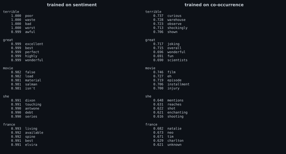
The collapse, stated precisely

Word	Sentiment-trained neighbours	Co-occurrence-trained neighbours
terrible	poor 1.000, waste 1.000, bad 1.000	curious 0.737, warehouse 0.728
great	excellent 0.999, best 0.999, perfect 0.999	joking 0.717, wonderful 0.696, fun 0.691
movie	false 0.982, load 0.982, material 0.981	film 0.746, episode 0.719, installment 0.706
france	living 0.993, available 0.992, spine 0.992	natalie 0.682, neo 0.673, tim 0.671

A cosine similarity of 1.000 between four different words means their vectors are parallel. The sentiment task is one-dimensional — a single number decides the output — so a 32-dimensional embedding trained on it only needs one useful direction, and words end up ordered along that axis with nothing else encoded. It classifies well (0.8562) and is useless as a general-purpose representation.

This is the precise reason downloaded embeddings exist. Word2Vec and GloVe are trained on co-occurrence over billions of tokens, so their similarity is “used in the same contexts” — a notion that transfers to tasks the original training never saw.

What frequency does to a vector

Times seen	Words	Nearest-neighbour similarity	Average similarity
3–10	300	0.6606	0.1661
10–30	300	0.6527	0.1698
30–100	300	0.6548	0.2137
100–1,000	300	0.6597	0.2302
1,000+	151	0.6177	0.1982

figure Skip-gram vectors, 1.6 million training pairs matplotlib

This figure exists because two earlier versions of it asserted a trend the data does not have. Nearest-neighbour similarity is flat — at 1.6 million pairs even a word seen five times finds *a* close neighbour. What frequency actually changes is the average column: frequent words drift towards the middle of the space, close to everything and specific to nothing. A rare word's vector is not obviously worse by this measure, which is a warning about the measure as much as about the vectors.

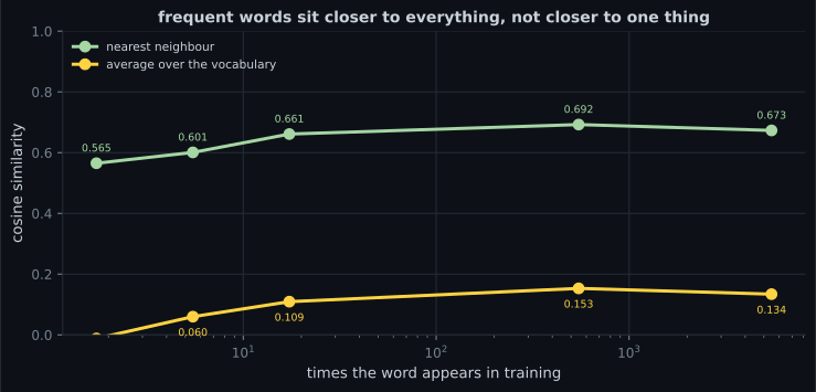
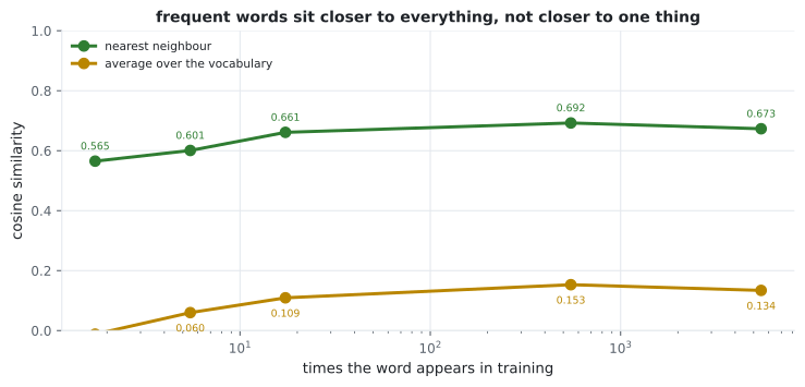
The honest reading: similarity statistics are a weak proxy for embedding quality. The strong test is a downstream task — the transfer-learning page used a linear probe for exactly this reason, and the same trick applies to word vectors.

Where the famous arithmetic comes from

$$\text{king} - \text{man} + \text{woman} \approx \text{queen}$$

This works on vectors trained on billions of tokens with a co-occurrence objective. It does not work here, and it is worth saying why rather than quietly omitting it: 8,000 reviews contain neither enough occurrences of the relevant words nor enough contexts to separate the relations. The analogy result is a property of scale, not of the algorithm — the algorithm on this page is the same one.

diagram Diagram mermaid

  flowchart TB
  A["what trains the vectors?"] --> B["a task label
(sentiment)"]
  A --> C["co-occurrence
(skip-gram, GloVe)"]
  B --> D["one useful direction
cosine 1.000 between synonyms"]
  D --> E["great for that task
useless elsewhere"]
  C --> F["many directions
movie/film 0.746"]
  F --> G["transfers to new tasks"]
  G --> H["at billions of tokens:
analogies, downloaded vectors"]

sketch Why a one-dimensional loss collapses an embedding p5.js Pause Restart

Drag the points. The loss only cares about their projection onto the sentiment axis, so gradient descent has no reason to keep them apart in any other direction.

sketch The measured table, ranked p5.js Pause Restart

Click a column to rank every row by it. The bars are that column's values and the highest and lowest are computed from the numbers, not written in.

Pitfalls

• Reading high cosine similarity as high quality. Four words at 1.000 means the space collapsed, not that the model understands synonymy.
• Reusing task-trained embeddings elsewhere. They encode one axis; france’s neighbours were living and spine.
• Expecting king − man + woman on a small corpus. That result comes from billions of tokens; the algorithm here is the same and the data is not.
• Judging vectors by similarity statistics. Nearest-neighbour similarity was flat across every frequency band — use a downstream probe instead.
• Paying for width without measuring it. 8 → 128 dimensions was 16× the matrix for +0.0350.
• Forgetting mask_zero=True. The padding row trains like any other and pollutes averages — measured on the masking page.
• Shuffling negatives in with positives after building them in blocks. An earlier run reported 0.4585 skip-gram accuracy — below chance — because validation_split took the last rows, which were all negatives.

Recap

• An embedding is a lookup table; the classifier on top of it here is 33 parameters against the matrix’s 256,000.
• Width buys little after 32 dimensions: 0.8253 → 0.8562 → 0.8602 for 8 → 32 → 128.
• Sentiment-trained vectors collapse onto one axis — cosine 1.000 between terrible, poor, waste and bad.
• Skip-gram on the same corpus found movie/film at 0.746 and movie/episode at 0.719 without ever seeing a label.
• Nearest-neighbour similarity was flat (0.62–0.66) across frequency bands; average similarity rose 0.1661 → 0.2302, so frequent words drift towards the centre.
• Analogy arithmetic is a property of corpus scale, not of the algorithm.

Next

Embeddings give words a shared space. The next page uses that space in the architecture that replaced recurrence: The Transformer Architecture.

pch.quizTag pch.quizDefaultTitle

1. Sentiment-trained embeddings put 'terrible', 'poor', 'waste' and 'bad' at cosine similarity 1.000. Why is that a problem?

   A It is not a problem — those words are synonyms B A similarity of 1.000 means the vectors are parallel: the space has collapsed onto the single axis the sentiment loss needs, so nothing else is encoded — 'france' ends up 0.99 from 'spine' C The similarity calculation is wrong D The embedding is too small
   pch.quizShowAnswer

   B — A similarity of 1.000 means the vectors are parallel: the space has collapsed onto the single axis the sentiment loss needs, so nothing else is encoded — 'france' ends up 0.99 from 'spine' — It classifies well (0.8562) and is useless as a general representation, which is exactly why downloaded co-occurrence embeddings exist.

2. Skip-gram on the same 8,000 reviews found movie/film at 0.746 without ever seeing a label. What signal did it use?

   A The sentiment of the surrounding review B Co-occurrence — it predicts whether two words appeared near each other, which forces it to distinguish words the label never needed to distinguish C The words' spelling D Document frequency, like TF-IDF
   pch.quizShowAnswer

   B — Co-occurrence — it predicts whether two words appeared near each other, which forces it to distinguish words the label never needed to distinguish — That notion of similarity — 'used in the same contexts' — is the one that transfers to tasks the training never saw.

3. Going from 8 to 128 embedding dimensions multiplied the matrix by 16 and improved accuracy by 0.0350. What does that suggest?

   A Always use the widest embedding you can afford B Most of the benefit arrives early — 8 to 32 was +0.0309 and 32 to 128 was +0.0040 — so width past a point is parameters spent on a lookup table C Embedding width does not matter D The model was underfitting at every width
   pch.quizShowAnswer

   B — Most of the benefit arrives early — 8 to 32 was +0.0309 and 32 to 128 was +0.0040 — so width past a point is parameters spent on a lookup table — Almost the entire model is the embedding matrix; the classifier on top was 33 parameters.

4. Nearest-neighbour similarity was flat (0.62-0.66) across every frequency band, while average similarity rose from 0.1661 to 0.2302. What is the right conclusion?

   A Rare words have better vectors B Similarity statistics are a weak proxy for quality — what frequency changes is how close a word sits to the whole vocabulary, not how sharp its nearest neighbour is C The vectors are untrained D The frequency bands were computed incorrectly
   pch.quizShowAnswer

   B — Similarity statistics are a weak proxy for quality — what frequency changes is how close a word sits to the whole vocabulary, not how sharp its nearest neighbour is — Two earlier versions of that figure asserted trends the data lacked. The strong test is a downstream probe, not a distance statistic.

5. Why does king - man + woman = queen not reproduce on this corpus?

   A Because skip-gram cannot represent analogies B Because the result depends on corpus scale — billions of tokens provide enough occurrences and contexts to separate the relations; 8,000 reviews do not C Because the embedding is only 32-dimensional D Because the arithmetic requires GloVe specifically
   pch.quizShowAnswer

   B — Because the result depends on corpus scale — billions of tokens provide enough occurrences and contexts to separate the relations; 8,000 reviews do not — The algorithm on this page is the same one used to produce those vectors. The difference is data, and saying so is more useful than omitting the experiment.

🧪 Try It Yourself

pch.exerciseTag pch.exerciseTitle

pch.exerciseTag pch.exerciseTitle

pch.exerciseTag pch.exerciseTitle

pch.exerciseTag pch.exerciseTitle

pch.exerciseTag pch.exerciseTitle