Backpropagation and Automatic Differentiation

Here is the function the book opens §5.6 with:

$$f(x) = \sqrt{x^2 + \exp(x^2)} + \cos\bigl(x^2 + \exp(x^2)\bigr) \tag{5.109}$$

and here is its derivative, written out:

$$\frac{\mathrm{d}f}{\mathrm{d}x} = 2x\left(\frac{1}{2\sqrt{x^2+\exp(x^2)}} - \sin\bigl(x^2+\exp(x^2)\bigr)\right)\bigl(1+\exp(x^2)\bigr) \tag{5.110}$$

The book’s comment: writing out the gradient in this explicit way is often impractical since it often results in a very lengthy expression for a derivative. In practice, it means that, if we are not careful, the implementation of the gradient could be significantly more expensive than computing the function.

And then the claim that makes the whole chapter land — the derivative costs about what the function costs, not more. The book calls that “quite counterintuitive” itself. This page counts the operations.

What you’ll learn

• §5.6.1: how the chain rule cascades through a $K$-layer network, Equations 5.111 to 5.118.
• §5.6.2: forward and reverse mode as two bracketings of the same product, Equations 5.119 to 5.121 — and why the shape of the Jacobian decides which is cheaper.
• Example 5.14 walked node by node, with the forward values of Equations 5.123–5.128 and the adjoints of Equations 5.135–5.142.
• What dropping the second term of Equation 5.137 costs: between $9.5\%$ and $47.8\%$, measured.
• The general algorithm, Equations 5.143 to 5.145, and why it is just the chain rule with bookkeeping.
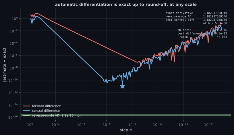
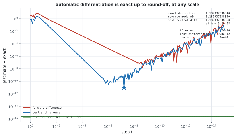
• Why AD beats finite differencing by five orders of magnitude on the same function, with no step size to tune.
• A measured look at vanishing gradients: $\lVert\nabla\rVert$ falling from $5.3\times10^{-1}$ to $3.9\times10^{-4}$ as depth goes $1 \to 16$.

Intuition: multiply the same factors in the other order

Take the book’s Figure 5.10 — data flowing $x \to a \to b \to y$. The chain rule says

$$\frac{\mathrm{d}y}{\mathrm{d}x} = \frac{\mathrm{d}y}{\mathrm{d}b}\frac{\mathrm{d}b}{\mathrm{d}a}\frac{\mathrm{d}a}{\mathrm{d}x} \tag{5.119}$$

Three factors, and matrix multiplication is associative, so you may bracket them either way:

$$\frac{\mathrm{d}y}{\mathrm{d}x} = \left(\frac{\mathrm{d}y}{\mathrm{d}b}\frac{\mathrm{d}b}{\mathrm{d}a}\right)\frac{\mathrm{d}a}{\mathrm{d}x} \tag{5.120}$$ $$\frac{\mathrm{d}y}{\mathrm{d}x} = \frac{\mathrm{d}y}{\mathrm{d}b}\left(\frac{\mathrm{d}b}{\mathrm{d}a}\frac{\mathrm{d}a}{\mathrm{d}x}\right) \tag{5.121}$$

Equation 5.120 accumulates from the output backwards — that is reverse mode, and it is backpropagation. Equation 5.121 accumulates from the input forwards — forward mode, gradients flowing with the data.

Same answer, same factors, different intermediate objects. And that is the entire difference: which partial products you have to store, and how big they are.

diagram Diagram mermaid

  flowchart TD
  CR["dy/dx = (dy/db)(db/da)(da/dx)
Eq 5.119 — three factors"]
  CR -->|"bracket from the LEFT"| REV["Eq 5.120: reverse mode
accumulate output → input
= backpropagation"]
  CR -->|"bracket from the RIGHT"| FWD["Eq 5.121: forward mode
accumulate input → output"]
  REV --> RC["cost: one sweep per OUTPUT
a scalar loss ⇒ ONE sweep"]
  FWD --> FC["cost: one sweep per INPUT
a million weights ⇒ a million sweeps"]
  RC --> WIN["reverse wins when n ≫ m
crossover at n = 3
a network: n in the millions, m = 1"]
  FC --> WIN
  REV --> ALG["the algorithm, Eq 5.143–5.145
forward: xᵢ = gᵢ(x_Pa(i))
seed: ∂f/∂x_D = 1
sweep: ∂f/∂xᵢ = Σ over CHILDREN"]
  ALG --> SUM["that Σ is the whole subtlety —
a node with two children needs
a SUM, not one product
(Eq 5.137)"]
  SUM --> COST["dropping one term: 9.5%–47.8% wrong"]

The math

§5.6.1 — the chain rule through a deep network

A deep network is an extreme case of composition:

$$\mathbf{y} = (f_K \circ f_{K-1} \circ \cdots \circ f_1)(\mathbf{x}) = f_K\bigl(f_{K-1}(\cdots(f_1(\mathbf{x}))\cdots)\bigr) \tag{5.111}$$

with each layer $f_i(\mathbf{x}_{i-1}) = \sigma(\mathbf{A}_{i-1}\mathbf{x}_{i-1} + \mathbf{b}_{i-1})$ for an activation $\sigma$ — logistic sigmoid, $\tanh$, or a rectified linear unit. Concretely:

$$\mathbf{f}_0 := \mathbf{x}, \qquad \mathbf{f}_i := \sigma_i(\mathbf{A}_{i-1}\mathbf{f}_{i-1} + \mathbf{b}_{i-1}),\quad i = 1,\dots,K \tag{5.112-5.113}$$

and we want the parameters $\boldsymbol{\theta} = \{\mathbf{A}_0,\mathbf{b}_0,\dots,\mathbf{A}_{K-1},\mathbf{b}_{K-1}\}$ minimising the squared loss

$$L(\boldsymbol{\theta}) = \lVert\mathbf{y} - \mathbf{f}_K(\boldsymbol{\theta},\mathbf{x})\rVert^2 \tag{5.114}$$

The chain rule then gives, layer by layer from the top:

$$\frac{\partial L}{\partial\boldsymbol{\theta}_{K-1}} = \frac{\partial L}{\partial\mathbf{f}_K}\frac{\partial\mathbf{f}_K}{\partial\boldsymbol{\theta}_{K-1}} \tag{5.115}$$ $$\frac{\partial L}{\partial\boldsymbol{\theta}_{K-2}} = \frac{\partial L}{\partial\mathbf{f}_K}\frac{\partial\mathbf{f}_K}{\partial\mathbf{f}_{K-1}}\frac{\partial\mathbf{f}_{K-1}}{\partial\boldsymbol{\theta}_{K-2}} \tag{5.116}$$ $$\frac{\partial L}{\partial\boldsymbol{\theta}_{K-3}} = \frac{\partial L}{\partial\mathbf{f}_K}\frac{\partial\mathbf{f}_K}{\partial\mathbf{f}_{K-1}}\frac{\partial\mathbf{f}_{K-1}}{\partial\mathbf{f}_{K-2}}\frac{\partial\mathbf{f}_{K-2}}{\partial\boldsymbol{\theta}_{K-3}} \tag{5.117}$$ $$\frac{\partial L}{\partial\boldsymbol{\theta}_i} = \frac{\partial L}{\partial\mathbf{f}_K}\frac{\partial\mathbf{f}_K}{\partial\mathbf{f}_{K-1}}\cdots\frac{\partial\mathbf{f}_{i+2}}{\partial\mathbf{f}_{i+1}}\frac{\partial\mathbf{f}_{i+1}}{\partial\boldsymbol{\theta}_i} \tag{5.118}$$

Look at what those four lines share. Every one of them starts with the same prefix, and each is the previous one with one more factor inserted. So computing them top-down means each layer reuses the product the layer above already formed — one new factor per layer, not a fresh product per layer. That reuse is backpropagation, and Equation 5.118 is the pattern it exploits.

§5.6.2 — automatic differentiation, in general

Equations 5.143 to 5.145

Let $x_1,\dots,x_d$ be the input variables, $x_{d+1},\dots,x_{D-1}$ the intermediate variables, and $x_D$ the output. The computation graph is

$$\text{For } i = d+1,\dots,D: \quad x_i = g_i\bigl(x_{\mathrm{Pa}(x_i)}\bigr) \tag{5.143}$$

where the $g_i$ are elementary functions and $x_{\mathrm{Pa}(x_i)}$ are the parent nodes of $x_i$. Since $f = x_D$,

$$\frac{\partial f}{\partial x_D} = 1 \tag{5.144}$$

and for the other variables,

$$\frac{\partial f}{\partial x_i} = \sum_{x_j\,:\,x_i\in\mathrm{Pa}(x_j)}\frac{\partial f}{\partial x_j}\frac{\partial x_j}{\partial x_i} = \sum_{x_j\,:\,x_i\in\mathrm{Pa}(x_j)}\frac{\partial f}{\partial x_j}\frac{\partial g_j}{\partial x_i} \tag{5.145}$$

Equation 5.143 is the forward propagation of the function; Equation 5.145 is the backpropagation of the gradient through the graph.

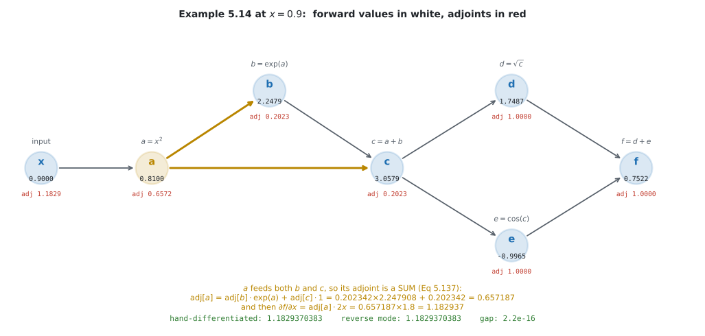
The one subtlety in the whole algorithm is that $\sum$. Most nodes have one child and their adjoint is a single product. A node with two children needs both terms — and that is Equation 5.137 in the worked example below.

The book’s scope note

Automatic differentiation applies to general computer programs and has forward and reverse modes. And on the choice: in the context of neural networks, where the input dimensionality is often much higher than the dimensionality of the labels, the reverse mode is computationally significantly cheaper than the forward mode.

From the book

Section 5.6. Equation 5.109 gives the example function and Equation 5.110 its explicit derivative, with the observation that writing gradients out this way is impractical and can make the gradient more expensive than the function. Section 5.6.1 covers deep networks: Equation 5.111 is the composition, 5.112–5.113 the layer definitions with $\sigma$ a sigmoid, $\tanh$ or ReLU, 5.114 the squared loss, and 5.115–5.118 the chain-rule cascade, illustrated by Figures 5.8 (forward) and 5.9 (backward). Section 5.6.2 introduces automatic differentiation as distinct from both symbolic differentiation and numerical approximation, cites Baydin et al. (2018), and uses Figure 5.10 to derive Equation 5.119 and its two bracketings — 5.120 reverse mode and 5.121 forward mode — noting that reverse mode is significantly cheaper when inputs outnumber labels. Example 5.14 (Equations 5.122–5.128) introduces the intermediate variables $a$ through $f$; Equations 5.129–5.134 give the elementary derivatives; Equations 5.135–5.142 walk the reverse sweep, including $\partial f/\partial a$ as a sum of two terms at Equation 5.137. The general algorithm is Equations 5.143–5.145, with Equation 5.144 seeding the sweep at 1.

Worked example by hand

Example 5.14, forward

Rather than evaluate Equation 5.109 as written, save work with intermediate variables:

$$a = x^2,\quad b = \exp(a),\quad c = a + b,\quad d = \sqrt{c},\quad e = \cos(c),\quad f = d + e \tag{5.123-5.128}$$

At $x = 0.9$:

variable	value
$a = x^2$	$0.810000000$
$b = \exp(a)$	$2.247907987$
$c = a+b$	$3.057907987$
$d = \sqrt{c}$	$1.748687504$
$e = \cos(c)$	$-0.996500481$
$f = d+e$	$0.752187023$

Six elementary operations, and note that $c$ is computed once and used twice — by $d$ and by $e$. That reuse is why the graph is a graph rather than a chain, and it is where the interesting frame is.

The elementary derivatives

$$\frac{\partial a}{\partial x} = 2x,\qquad \frac{\partial b}{\partial a} = \exp(a),\qquad \frac{\partial c}{\partial a} = 1 = \frac{\partial c}{\partial b} \tag{5.129-5.131}$$ $$\frac{\partial d}{\partial c} = \frac{1}{2\sqrt{c}},\qquad \frac{\partial e}{\partial c} = -\sin(c),\qquad \frac{\partial f}{\partial d} = 1 = \frac{\partial f}{\partial e} \tag{5.132-5.134}$$

Every one is a one-line school derivative. Nothing here is hard; the algorithm is in the order.

Example 5.14, backward

Working from the output:

$$\frac{\partial f}{\partial c} = \frac{\partial f}{\partial d}\frac{\partial d}{\partial c} + \frac{\partial f}{\partial e}\frac{\partial e}{\partial c} = 1\cdot\frac{1}{2\sqrt{c}} + 1\cdot(-\sin c) \tag{5.135, 5.139}$$ $$\frac{\partial f}{\partial b} = \frac{\partial f}{\partial c}\frac{\partial c}{\partial b} = \frac{\partial f}{\partial c}\cdot1 \tag{5.136, 5.140}$$ $$\boxed{\;\frac{\partial f}{\partial a} = \frac{\partial f}{\partial b}\frac{\partial b}{\partial a} + \frac{\partial f}{\partial c}\frac{\partial c}{\partial a} = \frac{\partial f}{\partial b}\exp(a) + \frac{\partial f}{\partial c}\cdot1\;} \tag{5.137, 5.141}$$ $$\frac{\partial f}{\partial x} = \frac{\partial f}{\partial a}\frac{\partial a}{\partial x} = \frac{\partial f}{\partial a}\cdot2x \tag{5.138, 5.142}$$

At $x = 0.9$:

adjoint	computation	value
$\partial f/\partial f$	seeded (Eq 5.144)	$1$
$\partial f/\partial d = \partial f/\partial e$	$1\cdot1$	$1$
$\partial f/\partial c$	$\tfrac{1}{2\sqrt{c}} - \sin c$	$0.202341706$
$\partial f/\partial b$	$0.202341706 \cdot 1$	$0.202341706$
$\partial f/\partial a$	$0.202341706\cdot2.247908 + 0.202341706$	$\mathbf{0.657187244}$
$\partial f/\partial x$	$0.657187244 \cdot 1.8$	$\mathbf{1.182937038}$

Against Equation 5.110 evaluated directly: $1.182937038340$ both ways, gap $2.2\times10^{-16}$.

Equation 5.137 is the frame to stop on

$a$ is the only node with two children — it feeds $b$ and it feeds $c$ — so its adjoint is a sum. Every other adjoint in this example is a single product, which is exactly why the sum is easy to forget.

Drop the second term and the answer is still plausible. Measured:

$x$	correct	with the second term dropped	relative error
$0.3$	$-0.58642666$	$-0.30639903$	$\mathbf{47.8\%}$
$0.6$	$-1.75775264$	$-1.03538738$	$41.1\%$
$0.9$	$1.18293704$	$0.81872197$	$30.8\%$
$1.2$	$9.93868781$	$8.03497839$	$19.2\%$
$1.5$	$27.78045491$	$25.13160340$	$9.5\%$

Right sign, right order of magnitude, wrong by up to half. And note the error is worst for small $x$ — so a gradient check on a small input is where it shows, which is the opposite of most numerical bugs.

The cost, counted

	operations
forward pass (Equations 5.123–5.128)	$6$
reverse sweep ($8$ graph edges, one multiply and one add each)	$16$
ratio	$\mathbf{2.67\times}$
Equation 5.110 evaluated as written	$11$, and it recomputes $x^2$ and $\exp(x^2)$

That is the book’s counterintuitive claim, made concrete. The derivative is $2.67$ times the function — a constant factor, not a blow-up — and the reason is that the reverse sweep reuses every forward value instead of recomputing it. Equation 5.110 does recompute them, which is exactly the “unnecessary overhead” the book warns about.

See it move

fieldExample 5.14, forward then backwardreverse-mode autodiff, §5.6

phase forwardx 0.9forward ops 0reverse ops 0

1# forward: evaluate every node in topological order2for i in d+1 .. D:  x_i = g_i(x_Pa(i))                       # Eq 5.1433 4# reverse: seed the output, then sweep backwards5adj[D] = 1                                                   # Eq 5.1446for i in D-1 .. 1:7    adj[i] = sum over children j of  adj[j] * d x_j / d x_i   # Eq 5.145

x0.90000000

Forward pass. The input is x = 0.9.

Play‹›1/14⟲

Six intermediates, then the sweep. Stop on the frame where a's adjoint is built: it is the only node with two children, so its adjoint is Equation 5.137's sum rather than a single product. The final frame checks the answer three independent ways.

fieldA scalar version of §5.6.1's deep networkreverse-mode autodiff, §5.6

phase forwardx 0.7forward ops 0reverse ops 0

1# forward: evaluate every node in topological order2for i in d+1 .. D:  x_i = g_i(x_Pa(i))                       # Eq 5.1433 4# reverse: seed the output, then sweep backwards5adj[D] = 1                                                   # Eq 5.1446for i in D-1 .. 1:7    adj[i] = sum over children j of  adj[j] * d x_j / d x_i   # Eq 5.145

x0.70000000

Forward pass. The input is x = 0.7.

Play‹›1/14⟲

Two tanh layers and a squared loss. The adjoints arriving at each weight are exactly what backpropagation computes, and the operation counts show the reverse sweep costing twice the forward pass.

sketch Forward mode or reverse mode? p5.js Pause Restart

Drag the input and output widths. Forward mode needs one sweep per input, reverse mode one per output, so the cheaper choice is decided by the shape of the Jacobian and nothing else. The star marks where a neural network sits: millions of inputs, one scalar loss.

sketch Vanishing gradients, measured p5.js Pause Restart

A K-layer tanh network with a squared loss. Drag the depth and watch the gradient norm collapse: each layer multiplies by a tanh derivative no bigger than 1, so K of them compound. This is the reason deep networks were hard before ReLU and residual connections, and it falls straight out of Equation 5.118's product.

From scratch

autodiff_from_scratch.py

import numpy as np
 
def f_5_14(x):
    """Eq 5.109, via the intermediates of Eq 5.123-5.128."""
    a = x ** 2
    b = np.exp(a)
    c = a + b
    d = np.sqrt(c)
    e = np.cos(c)
    return d + e
 
def dfdx_closed(x):
    """Eq 5.110, the book's explicit gradient."""
    u = x ** 2 + np.exp(x ** 2)
    return 2 * x * (1 / (2 * np.sqrt(u)) - np.sin(u)) * (1 + np.exp(x ** 2))
 
def reverse_5_14(x):
    """Forward pass, then Eq 5.135-5.142."""
    a = x ** 2                                          # Eq 5.123
    b = np.exp(a)                                       # Eq 5.124
    c = a + b                                           # Eq 5.125
    d = np.sqrt(c)                                      # Eq 5.126
    e = np.cos(c)                                       # Eq 5.127
    f = d + e                                           # Eq 5.128
 
    adj_f = 1.0                                         # Eq 5.144
    adj_d = adj_f * 1.0                                 # Eq 5.134
    adj_e = adj_f * 1.0
    adj_c = adj_d * (1 / (2 * np.sqrt(c))) + adj_e * (-np.sin(c))    # Eq 5.135
    adj_b = adj_c * 1.0                                             # Eq 5.136
    adj_a = adj_b * np.exp(a) + adj_c * 1.0                         # Eq 5.137 <- a SUM
    adj_x = adj_a * 2 * x                                           # Eq 5.138
    return dict(a=a, b=b, c=c, d=d, e=e, f=f,
                adj_c=adj_c, adj_b=adj_b, adj_a=adj_a, adj_x=adj_x)
 
x0 = 0.9
st = reverse_5_14(x0)
print(f"forward pass at x = {x0}   (Eq 5.123-5.128)")
for k in ("a", "b", "c", "d", "e", "f"):
    print(f"  {k} = {st[k]:.9f}")
print()
print("reverse sweep (Eq 5.135-5.142)")
print(f"  adj[c] = 1*(1/(2*sqrt(c))) + 1*(-sin(c)) = {st['adj_c']:.9f}")
print(f"  adj[b] = adj[c]*1                        = {st['adj_b']:.9f}")
print(f"  adj[a] = adj[b]*exp(a) + adj[c]*1        = {st['adj_a']:.9f}   <- a SUM, Eq 5.137")
print(f"  adj[x] = adj[a]*2x                       = {st['adj_x']:.9f}")
print()
print(f"Eq 5.110 (the explicit gradient)             {dfdx_closed(x0):.12f}")
print(f"reverse mode                                 {st['adj_x']:.12f}")
print(f"gap                                          {abs(st['adj_x'] - dfdx_closed(x0)):.1e}")
 
print()
print("what dropping the second term of Eq 5.137 costs")
for x in (0.3, 0.6, 0.9, 1.2, 1.5):
    a = x ** 2
    b = np.exp(a)
    c = a + b
    adj_c = (1 / (2 * np.sqrt(c))) + (-np.sin(c))
    full = (adj_c * np.exp(a) + adj_c * 1.0) * 2 * x
    dropped = (adj_c * np.exp(a)) * 2 * x
    exact = dfdx_closed(x)
    print(f"  x = {x:<4}  full {full:>13.8f}   dropping the second term {dropped:>13.8f}"
          f"   relative error {abs(dropped - exact) / abs(exact):>8.1%}")

output

forward pass at x = 0.9   (Eq 5.123-5.128)
  a = 0.810000000
  b = 2.247907987
  c = 3.057907987
  d = 1.748687504
  e = -0.996500481
  f = 0.752187023
 
reverse sweep (Eq 5.135-5.142)
  adj[f] = 1
  adj[d] = adj[e] = 1
  adj[c] = 1*(1/(2*sqrt(c))) + 1*(-sin(c)) = 0.202341706
  adj[b] = adj[c]*1                        = 0.202341706
  adj[a] = adj[b]*exp(a) + adj[c]*1        = 0.657187244   <- a SUM, Eq 5.137
  adj[x] = adj[a]*2x                       = 1.182937038
 
Eq 5.110 (the explicit gradient)             1.182937038340
reverse mode                                 1.182937038340
gap                                          2.2e-16
 
what dropping the second term of Eq 5.137 costs
  x = 0.3   full   -0.58642666   dropping the second term   -0.30639903   relative error    47.8%
  x = 0.6   full   -1.75775264   dropping the second term   -1.03538738   relative error    41.1%
  x = 0.9   full    1.18293704   dropping the second term    0.81872197   relative error    30.8%
  x = 1.2   full    9.93868781   dropping the second term    8.03497839   relative error    19.2%
  x = 1.5   full   27.78045491   dropping the second term   25.13160340   relative error     9.5%

On real data

figure The book's Figure 5.11, with numbers on it matplotlib

Example 5.14 at x = 0.9. The forward values reproduce Equations 5.123 to 5.128 and the adjoints reproduce 5.135 to 5.142. The highlighted node is a, the only one with two children — its adjoint is 0.202342 times 2.247908 plus 0.202342, which is 0.657187, and then df/dx is that times 1.8.

figure Which mode, decided by the Jacobian's shape matplotlib

With a scalar loss, forward mode needs n sweeps and reverse mode one, so reverse wins from n = 3. The heatmap generalises it: the choice depends only on whether inputs or outputs are more numerous. The star marks a network — many in, one out — which is the corner reverse mode was built for.

figure Automatic differentiation has no step size matplotlib

The derivative of Example 5.14 three ways. AD lands at 2.2e-16 and does not depend on h at all; over 200 values of h the best central difference reaches only 9.8e-12, at h = 5.8e-08 — a factor of forty thousand worse, and that is the BEST h, which you do not know in advance.

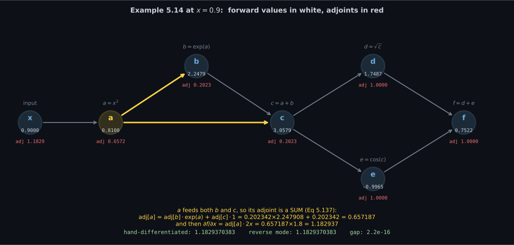
Reading the plot

From the graph figure. Follow the red numbers right to left. They start at $1$ — Equation 5.144’s seed — and every node multiplies by one local derivative as the sweep passes. Six of the seven nodes have a single incoming red edge, so their adjoint is one product. The seventh is $a$, and its box is where the sum happens.

The number to check is $0.657187$. Both contributions come from the same $\partial f/\partial c = 0.202342$: one routed through $b$ and scaled by $\exp(a) = 2.247908$, one routed directly through $c$ and scaled by $1$. Add them and you get $0.454846 + 0.202342 = 0.657187$. Multiply by $2x = 1.8$ and you have the answer.

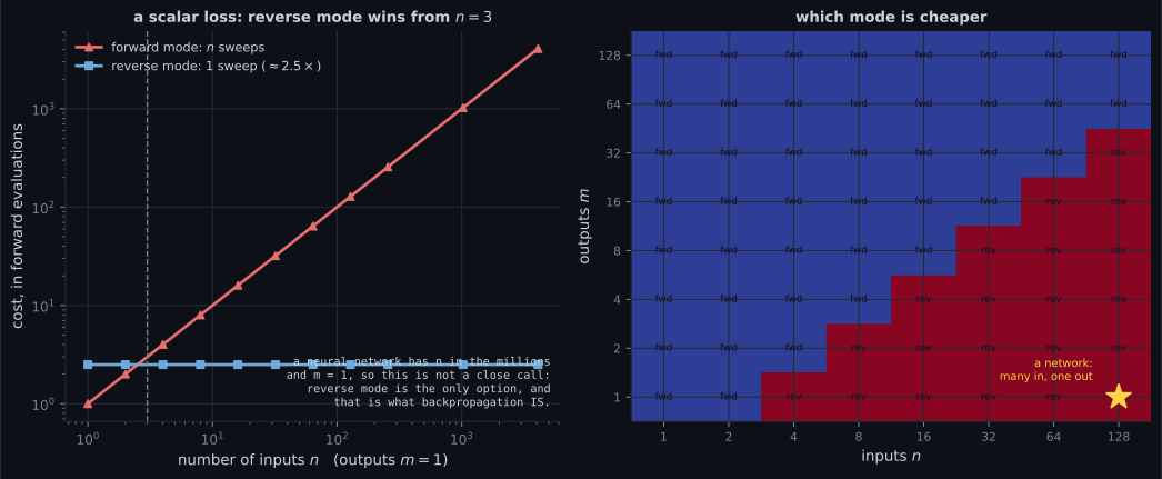
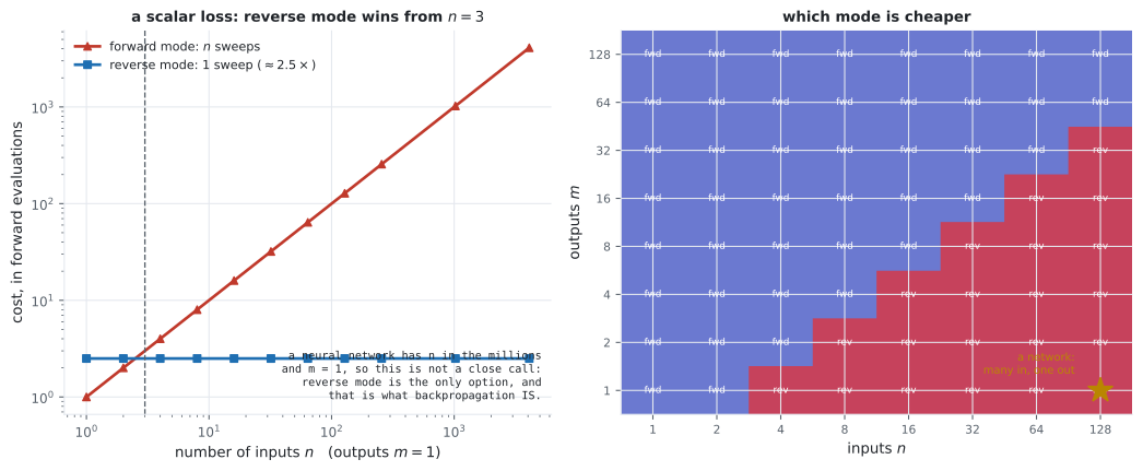
From the cost figure. The left panel’s two lines cross at $n = 3$ and never come back. That is the whole argument for backpropagation, and it does not depend on anything about the function — only on the shape of its Jacobian.

The heatmap makes the rule general: forward mode costs one sweep per input, reverse mode one per output. So the question is never “which is better”, it is “which dimension is bigger”. A Jacobian-vector product wants forward mode; a scalar loss wants reverse. A network has a million-plus inputs and one output, which is why reverse mode is not a preference there but the only option.

From the accuracy figure. The flat green line is the point: AD has no $h$, so it has no V. Its error is $2.2\times10^{-16}$ — one rounding — and it is the same at every scale.

The comparison worth quoting is against the best possible difference:

method	best error	at
forward difference	$1.7\times10^{-8}$	$h = 2.1\times10^{-9}$
central difference	$9.8\times10^{-12}$	$h = 5.8\times10^{-8}$
reverse-mode AD	$\mathbf{2.2\times10^{-16}}$	no $h$

Four orders of magnitude better than the best central difference — and you do not get to pick the best $h$ in advance. On a coarser grid of sixteen step sizes the best central difference is $9.6\times10^{-11}$, which is $4.3\times10^{5}$ times worse than AD. That factor is why nobody trains with finite differences and why gradient checking is a debugging tool rather than a method.

Pitfalls

A node with two children needs a sum, and forgetting it looks plausible

Equation 5.137 has two terms because $a$ feeds both $b$ and $c$. Drop one and the gradient is still the right sign and the right order of magnitude — measured between $9.5\%$ and $47.8\%$ wrong across $x \in [0.3, 1.5]$. The error is worst for small $x$, so a gradient check on a small input catches it and one on a large input may not.

Never train with finite differences

Two independent reasons. Accuracy: the best central difference on Example 5.14 is $9.8\times10^{-12}$ against AD’s $2.2\times10^{-16}$, and you have to know the best $h$ to get it. Cost: a gradient by differencing needs $2n$ function evaluations, so at $n$ parameters it is $O(n)$ times a forward pass while reverse mode is $O(1)$ times one. At a million parameters that is a factor of a million.

Forward mode is not the worse mode, it is the mode for a different shape

Reverse mode costs one sweep per output. For a function with one input and many outputs — a curve’s velocity, a sensitivity to one hyperparameter — forward mode is strictly cheaper, and the crossover measured here is at $n = 3$. The book states this as a fact about neural networks specifically, not about the modes.

Reverse mode has to store the forward pass

The reuse that makes the derivative cheap in time is what makes it expensive in memory: every intermediate value has to survive until the sweep reaches it. That is the actual constraint on training large models, and it is why gradient checkpointing exists — recompute some intermediates instead of storing them, trading the $2.67\times$ time factor up in exchange for less memory.

Vanishing gradients are a property of the product, not of the algorithm

Equation 5.118 says the gradient at layer $i$ is a product of $K - i$ Jacobians. With $\tanh$, every factor has magnitude at most $1$, so the product can only shrink. Measured on a scalar chain: the gradient norm falls from $5.30\times10^{-1}$ at $K = 1$ to $3.87\times10^{-4}$ at $K = 16$. Backpropagation is computing the right answer; the right answer is small.

Compare

method	exactness	cost of one gradient	needs
by hand (Eq 5.110)	exact	your time; and it recomputed $x^2$ and $\exp(x^2)$	a closed form
forward difference	$O(h)$, floor $\approx10^{-8}$	$n + 1$ evaluations	nothing
central difference	$O(h^2)$, floor $\approx10^{-11}$	$2n$ evaluations	nothing
forward-mode AD	machine precision	$n$ sweeps	the code
reverse-mode AD	machine precision	$m$ sweeps, $\approx2.67\times$ one pass	the code, plus memory for the tape
symbolic	exact	expression grows with depth	a closed form

The two AD rows are the same algorithm bracketed differently — Equations 5.120 and 5.121 — and the choice between them is arithmetic on $m$ and $n$, not judgement.

pch.quizTag Check your understanding

1. Forward and reverse mode are described as differing 'in the order of multiplication'. What exactly is being reordered?

   A The order the layers are evaluated B The bracketing of one product of Jacobians. Matrix multiplication is associative, so (dy/db · db/da) · da/dx and dy/db · (db/da · da/dx) give the same answer — Equations 5.120 and 5.121 — with different intermediate objects C The order the parameters are updated D Whether the derivative is exact
   pch.quizShowAnswer

   B — The bracketing of one product of Jacobians. Matrix multiplication is associative, so (dy/db · db/da) · da/dx and dy/db · (db/da · da/dx) give the same answer — Equations 5.120 and 5.121 — with different intermediate objects — Same factors, same answer, different partial products to store. Reverse mode accumulates from the output and so pays one sweep per output; forward mode accumulates from the input and pays one per input.

2. Why is reverse mode the only practical choice for training a network?

   A It is more accurate B Because the cost is one sweep per OUTPUT, and a loss is one scalar — while forward mode would need one sweep per parameter. The crossover measured here is n = 3, and a network has millions of parameters C Because forward mode cannot handle nonlinearities D Because it uses less memory
   pch.quizShowAnswer

   B — Because the cost is one sweep per OUTPUT, and a loss is one scalar — while forward mode would need one sweep per parameter. The crossover measured here is n = 3, and a network has millions of parameters — Note the last option is backwards: reverse mode uses MORE memory, because every intermediate has to survive until the sweep reaches it. That is why gradient checkpointing exists.

3. Equation 5.137 is a sum of two terms. What happens if you keep only the first?

   A The gradient is off by a sign B The gradient stays the right sign and order of magnitude but is wrong by between 9.5 and 47.8 percent, worst for small x — plausible enough to pass a casual check C The computation fails D Nothing, the second term is zero
   pch.quizShowAnswer

   B — The gradient stays the right sign and order of magnitude but is wrong by between 9.5 and 47.8 percent, worst for small x — plausible enough to pass a casual check — a is the only node in Example 5.14 with two children, so it is the only adjoint that is a sum rather than a single product — which is exactly why it is easy to forget. And the error being worst for SMALL x inverts the usual debugging instinct.

4. The reverse sweep on Example 5.14 costs 16 operations against the forward pass's 6. Why is that the interesting number?

   A Because 16 is small B Because it is a constant factor — 2.67x — rather than a blow-up, which is the book's counterintuitive claim. Equation 5.110 written out is 11 operations AND recomputes x-squared and exp(x-squared) that the forward pass already had C Because it beats finite differences D Because 8 edges is the graph size
   pch.quizShowAnswer

   B — Because it is a constant factor — 2.67x — rather than a blow-up, which is the book's counterintuitive claim. Equation 5.110 written out is 11 operations AND recomputes x-squared and exp(x-squared) that the forward pass already had — The reuse is the mechanism: the reverse sweep reads forward values instead of recomputing them. Symbolic differentiation does recompute them, which is the 'unnecessary overhead' the book warns about at Equation 5.110.

5. The gradient norm fell from 5.3e-01 at depth 1 to 3.9e-04 at depth 16. Is backpropagation losing accuracy?

   A Yes, error accumulates over layers B No. Equation 5.118 makes the gradient at layer i a product of K minus i Jacobians, and every tanh derivative has magnitude at most 1 — so the product can only shrink. The algorithm is exact; the answer is genuinely small C Yes, because of round-off D No, the measurement is wrong
   pch.quizShowAnswer

   B — No. Equation 5.118 makes the gradient at layer i a product of K minus i Jacobians, and every tanh derivative has magnitude at most 1 — so the product can only shrink. The algorithm is exact; the answer is genuinely small — Measured against finite differences the reverse-mode gradient agrees to 6.8e-08 even at depth 16, so it is computing correctly. Vanishing gradients are a property of the product that Eq 5.118 describes, which is why ReLU (derivative exactly 1 when active) and residual connections both attack the factors rather than the algorithm.

🧪 Try It Yourself

Exercise 1 – Example 5.14, forward and backward

pch.exerciseTag pch.exerciseTitle

Exercise 2 – What dropping Equation 5.137’s second term costs

pch.exerciseTag pch.exerciseTitle

Exercise 3 – AD against differencing, at every step size

pch.exerciseTag pch.exerciseTitle

Exercise 4 – Reverse mode on a deep chain, and vanishing gradients

pch.exerciseTag pch.exerciseTitle

Exercise 5 – Count the operations

pch.exerciseTag pch.exerciseTitle

Recall card

• Forward and reverse mode are the same product bracketed differently — Equations 5.120 and 5.121. Same factors, same answer, different intermediates to store.
• Reverse mode costs one sweep per OUTPUT, forward mode one per INPUT. With a scalar loss the crossover is n = 3, and a network has millions of parameters — so reverse mode is not a preference there, it is the only option.
• Equation 5.145’s sum is the whole subtlety. A node with one child has a single-product adjoint; a node with two children needs both terms.
• Example 5.14’s node a is the only one with two children, so Equation 5.137 is the only sum. Dropping one term leaves the gradient the right sign and order of magnitude but 9.5 to 47.8 percent wrong — worst for SMALL x.
• The derivative costs a constant factor of the function, not a blow-up. Measured: 6 forward operations against 16 in the reverse sweep — 2.67x — because the sweep reuses forward values instead of recomputing them.
• Equation 5.110 written out is 11 operations and recomputes x-squared and exp(x-squared), which is exactly the “unnecessary overhead” the book warns about.
• AD has no step size, so no V-shaped error curve. Measured: 2.2e-16 against a best central difference of 9.8e-12 over 200 step sizes — and you must already know the best h to get that.
• Reverse mode trades memory for time. Every intermediate must survive until the sweep reaches it, which is the real constraint on training and the reason gradient checkpointing exists.
• Vanishing gradients come from Equation 5.118’s product, not from the algorithm. Measured on a tanh chain: the gradient norm falls from 5.30e-01 at depth 1 to 3.87e-04 at depth 16, while still agreeing with finite differences to 6.8e-08.
• §5.6.1’s cascade reuses its own prefix. Equations 5.115 to 5.118 each extend the previous product by one factor, and exploiting that reuse is what backpropagation is.

Next: Higher-Order Derivatives — the Hessian, and the question the gradient cannot answer.