The Latent Variable Perspective

Six sections of PCA and not one probability. §10.7 adds one, and the book is direct about why:

On the one hand, this approach may be appealing as it allows us to sidestep all the mathematical difficulties that come with probability theory, but on the other hand, a probabilistic model would offer us more flexibility and useful insights.

The payoff list is eight items long, and it is the same list Chapter 9 earned by going from §9.2 to §9.3: a likelihood, model comparison by marginal likelihood, a generative model, missing data by Bayes’ theorem, and a notion of novelty.

What you’ll learn

• Equations 10.63–10.66: the generative process, and what it means that the arrow points from $\mathbf{z}$ to $\mathbf{x}$.
• Equations 10.69–10.70b: $p(\mathbf{x}) = \mathcal{N}(\boldsymbol\mu,\ \mathbf{B}\mathbf{B}^\top + \sigma^2\mathbf{I})$ — checked by $400{,}000$ ancestral samples, agreeing to $2.1\times10^{-3}$ relative, the Monte-Carlo floor.
• Equation 10.71: the cross-covariance $\mathrm{Cov}[\mathbf{x},\mathbf{z}]$ is exactly $\mathbf{B}$.
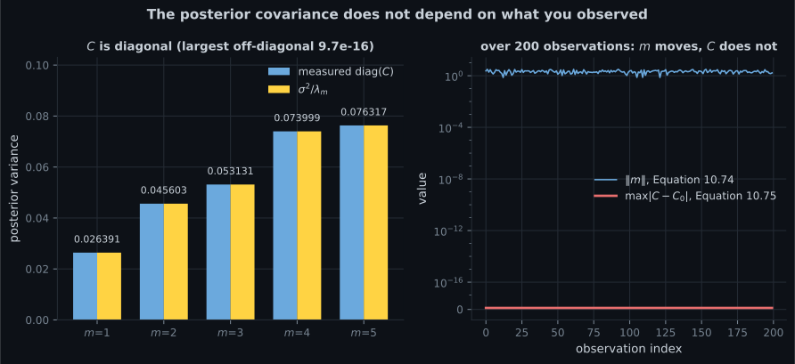
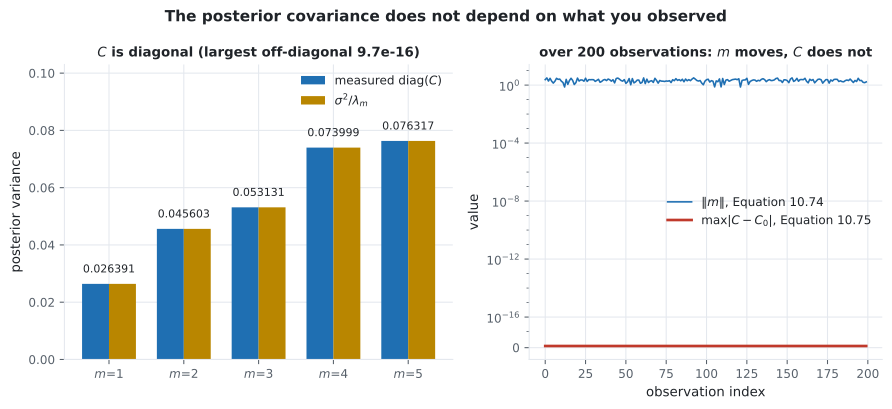
• Equations 10.73–10.75: the posterior over the code. $\mathbf{C}$ does not depend on $\mathbf{x}$ — measured, exactly $0$ change across $200$ observations — which is the same structural fact page 907 measured for $\mathbf{S}_N$.
• A closed form the book does not give: $\mathbf{C} = \sigma^2(\mathbf{B}^\top\mathbf{B} + \sigma^2\mathbf{I})^{-1}$, which for the ML $\mathbf{B}$ is diagonal with entries $\sigma^2/\lambda_m$ — measured to $9.7\times10^{-16}$.
• Equations 10.77–10.79: $\sigma^2_{\mathrm{ML}}$ is page 1004’s $J_M$ divided by $D-M$, matched to eight decimals.
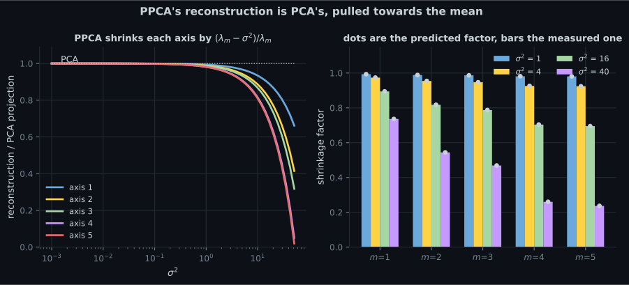
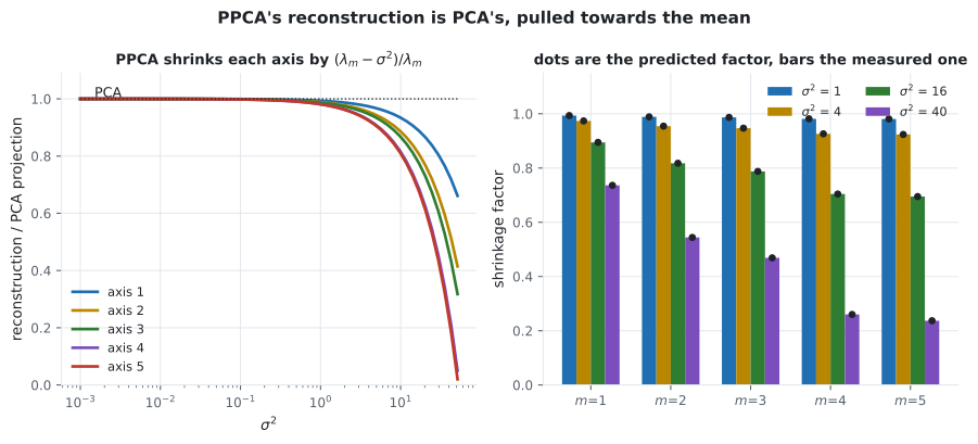
• PPCA is PCA with shrinkage. The reconstruction is the PCA projection scaled by $(\lambda_m-\sigma^2)/\lambda_m$ on each axis — measured to six decimals at four noise levels — and converges to PCA as $\sigma\to0$.

Intuition: PCA describes the data, PPCA claims to have made it

Everything before this page is a statement about a dataset you already have: here is the subspace that keeps the most variance. Nothing in it says what a new image would look like, or how surprised you should be by one.

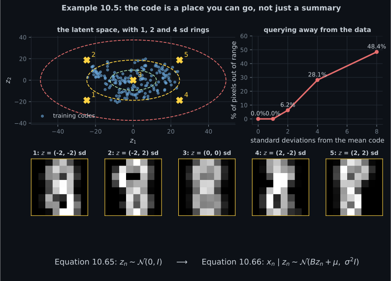
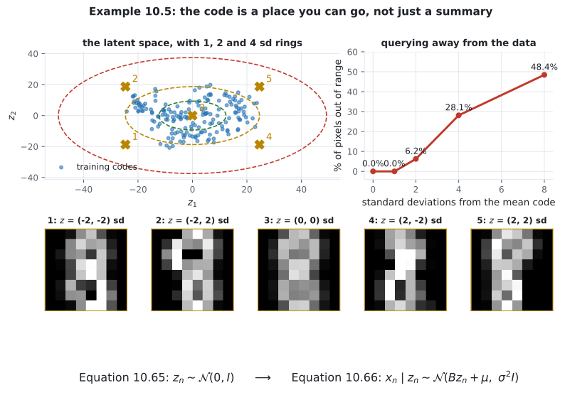
PPCA writes down a story instead. Draw $\mathbf{z}$ from a standard Gaussian; push it through an affine map; add noise. That story assigns a probability to every point in $\mathbb{R}^D$, which is what buys the eight items on the list — and it also commits you to claims that can be wrong.

diagram The generative direction, and the inference that reverses it mermaid

  flowchart LR
  Z["z ~ N(0, I)
Equation 10.65"] -->|"B z + mu"| XM["the mean of x"]
  XM -->|"+ noise, sigma^2 I"| X["x, Equation 10.66"]
  X -.->|"Bayes: Equations 10.73 to 10.75"| POST["p(z | x) = N(m, C)
C has no x in it"]
  Z --> J["the joint, Equation 10.72
cross-covariance exactly B"]
  X --> J
  J --> MARG["p(x) = N(mu, BB' + sigma^2 I)
Equations 10.69, 10.70b"]

§10.7.1 The generative process

$$\mathbf{x} = \mathbf{B}\mathbf{z} + \boldsymbol\mu + \boldsymbol\epsilon \in \mathbb{R}^D, \qquad \boldsymbol\epsilon \sim \mathcal{N}(\mathbf{0}, \sigma^2\mathbf{I}) \qquad \text{(10.63)}$$ $$\mathbf{z}_n \sim \mathcal{N}(\mathbf{z} \mid \mathbf{0}, \mathbf{I}), \qquad \mathbf{x}_n \mid \mathbf{z}_n \sim \mathcal{N}(\mathbf{x} \mid \mathbf{B}\mathbf{z}_n + \boldsymbol\mu, \sigma^2\mathbf{I}) \qquad \text{(10.65), (10.66)}$$

This is ancestral sampling: draw the parent, then the child.

The direction of the arrow is a claim, not a convention

The arrow points from $\mathbf{z}$ to $\mathbf{x}$, which means that the PPCA model assumes a lower-dimensional latent cause $\mathbf{z}$ for high-dimensional observations $\mathbf{x}$.

Compare page 807’s directed graphical models. PCA computed $\mathbf{z} = \mathbf{B}^\top\mathbf{x}$ — a function of the data, pointing the other way. PPCA asserts the reverse and then derives $\mathbf{z}$-given-$\mathbf{x}$ by Bayes’ theorem, “to ‘invert’ the arrow implicitly”.

The two happen to give almost the same answer here. They would not for a nonlinear map, and the whole of variational autoencoders lives in that gap.

figure Example 10.5: the latent space is somewhere you can go matplotlib

Every point in the plane decodes to an image, not just the ones the data occupies. The right panel measures the book's remark that querying away from the data produces artifacts: at two standard deviations 6.2 percent of the generated pixels fall outside the range any real image can occupy, at four 28.1 percent, at eight 48.4 percent.

§10.7.2 The likelihood, and why it needs the integral

The conditional $p(\mathbf{x}\mid\mathbf{z})$ cannot be maximised over parameters, because it still mentions $\mathbf{z}$. Integrating it out:

$$p(\mathbf{x}\mid\mathbf{B},\boldsymbol\mu,\sigma^2) = \int \mathcal{N}(\mathbf{x}\mid\mathbf{B}\mathbf{z}+\boldsymbol\mu,\sigma^2\mathbf{I})\,\mathcal{N}(\mathbf{z}\mid\mathbf{0},\mathbf{I})\,\mathrm{d}\mathbf{z} \qquad \text{(10.68b)}$$ $$\mathbb{E}[\mathbf{x}] = \boldsymbol\mu, \qquad \mathbb{V}[\mathbf{x}] = \mathbf{B}\mathbf{B}^\top + \sigma^2\mathbf{I} \qquad \text{(10.69), (10.70b)}$$

Verified by running Equations 10.65 and 10.66 forward $400{,}000$ times with $M = 5$, $\sigma^2 = 4$:

	value
$\lVert$empirical mean $-\ \boldsymbol\mu\rVert$	$0.037050$
$\max\lvert$empirical covariance $-\ (\mathbf{B}\mathbf{B}^\top+\sigma^2\mathbf{I})\rvert$	$0.065452$
the same, relative to the largest entry	$2.1\times10^{-3}$
Monte-Carlo floor, $1/\sqrt{K}$	$1.6\times10^{-3}$

The gap is sampling noise of the size you would predict, not a discrepancy.

The joint, using $\mathrm{Cov}[\mathbf{x},\mathbf{z}] = \mathbf{B}\,\mathrm{Cov}_z[\mathbf{z},\mathbf{z}] = \mathbf{B}$ (Equation 10.71):

$$p(\mathbf{x},\mathbf{z}\mid\mathbf{B},\boldsymbol\mu,\sigma^2) = \mathcal{N}\!\left(\begin{bmatrix}\mathbf{x}\\ \mathbf{z}\end{bmatrix}\ \Bigg|\ \begin{bmatrix}\boldsymbol\mu\\ \mathbf{0}\end{bmatrix},\ \begin{bmatrix}\mathbf{B}\mathbf{B}^\top+\sigma^2\mathbf{I} & \mathbf{B}\\ \mathbf{B}^\top & \mathbf{I}\end{bmatrix}\right) \qquad \text{(10.72)}$$

§10.7.3 The posterior, and the thing it does not look at

Gaussian conditioning (§6.5.1) gives

$$p(\mathbf{z}\mid\mathbf{x}) = \mathcal{N}(\mathbf{z}\mid\mathbf{m},\mathbf{C}) \qquad \text{(10.73)}$$ $$\mathbf{m} = \mathbf{B}^\top(\mathbf{B}\mathbf{B}^\top+\sigma^2\mathbf{I})^{-1}(\mathbf{x}-\boldsymbol\mu) \qquad \text{(10.74)}$$ $$\mathbf{C} = \mathbf{I} - \mathbf{B}^\top(\mathbf{B}\mathbf{B}^\top+\sigma^2\mathbf{I})^{-1}\mathbf{B} \qquad \text{(10.75)}$$

Note that the posterior covariance does not depend on the observed data $\mathbf{x}$.

figure The measured posterior covariance, and what it is made of matplotlib

Left: the diagonal of C against sigma-squared over lambda-m, which is what the Woodbury form reduces to for the maximum-likelihood B. Right: over 200 different observations the posterior mean moves and the posterior covariance changes by exactly zero. Page 907 measured the same structure for the Bayesian linear-regression posterior.

A closed form the book does not give, and what it says

Equation 10.75 inverts a $D\times D$ matrix for an $M$-dimensional posterior — the same shape of inefficiency page 908 found in Equation 9.64. Woodbury again:

$$\mathbf{C} = \sigma^2\left(\mathbf{B}^\top\mathbf{B} + \sigma^2\mathbf{I}\right)^{-1}$$

Measured against Equation 10.75: $9.7\times10^{-16}$. And now the structure is readable. For the maximum-likelihood $\mathbf{B} = \mathbf{T}(\boldsymbol\Lambda-\sigma^2\mathbf{I})^{1/2}$ we have $\mathbf{B}^\top\mathbf{B} = \boldsymbol\Lambda - \sigma^2\mathbf{I}$, so

$$\mathbf{C} = \sigma^2\boldsymbol\Lambda^{-1}, \qquad C_{mm} = \frac{\sigma^2}{\lambda_m}$$

$m$	measured $C_{mm}$	$\sigma^2/\lambda_m$
$1$	$0.026391$	$0.026391$
$2$	$0.045603$	$0.045603$
$3$	$0.053131$	$0.053131$
$4$	$0.073999$	$0.073999$
$5$	$0.076317$	$0.076317$

Largest off-diagonal entry: $9.7\times10^{-16}$, and the mean $\mathbf{m}$ ranges over $0.7394$ to $3.1530$ in norm across the dataset while $\mathbf{C}$ never moves. The posterior is uncertain in inverse proportion to how much variance the axis carries — which is the quantitative version of “the later components are less reliable”, and it needs no data to state.

§10.8’s maximum-likelihood parameters

$$\boldsymbol\mu_{\mathrm{ML}} = \frac{1}{N}\sum_{n=1}^{N}\mathbf{x}_n, \qquad \mathbf{B}_{\mathrm{ML}} = \mathbf{T}(\boldsymbol\Lambda-\sigma^2\mathbf{I})^{\frac12}\mathbf{R}, \qquad \sigma^2_{\mathrm{ML}} = \frac{1}{D-M}\sum_{j=M+1}^{D}\lambda_j \qquad \text{(10.77)–(10.79)}$$

Equation 10.79 is page 1004’s $J_M$ divided by the number of directions it is spread across — “the average leftover variance that we cannot capture with the first $M$ principal components is treated as observation noise.” Measured:

$M$	$\sigma^2_{\mathrm{ML}}$	$J_M/(D-M)$
$1$	$9.35857873$	$9.35857873$
$5$	$5.42581981$	$5.42581981$
$10$	$3.07760746$	$3.07760746$
$20$	$1.34890465$	$1.34890465$
$40$	$0.12051166$	$0.12051166$

Two consequences worth stating:

$\mathbf{R}$ is back. Equation 10.78 ends in “an arbitrary orthogonal matrix”, which page 1004 measured: rotating $\mathbf{B}$ leaves the reconstruction error at $320.123369$ and the projector identical to $1.1\times10^{-16}$. Here it means the maximum-likelihood solution is a whole family, and “PCA can identify the best lower-dimensional subspace in which the signals live, but not the signals themselves” (§10.8). ICA exists to break that tie by making $p(\mathbf{z})$ non-Gaussian.

The margin note is a guarantee, not an observation. $\boldsymbol\Lambda-\sigma^2\mathbf{I}$ is positive semi-definite because $\sigma^2_{\mathrm{ML}}$ is an average of the discarded eigenvalues, and the discarded ones are all below the kept ones by construction. The square root in Equation 10.78 is always real.

PPCA is PCA with shrinkage

Substituting $\mathbf{B}_{\mathrm{ML}}$ into Equation 10.74 and reconstructing gives, per axis,

$$\frac{(\mathbf{B}\mathbf{m})_m}{(\text{PCA projection})_m} = \frac{\lambda_m - \sigma^2}{\lambda_m}$$

Measured against the prediction, four noise levels, five axes, and every cell matches:

$\sigma^2$	axis $1$	axis $2$	axis $3$	axis $4$	axis $5$
$1$	$0.993402$	$0.988599$	$0.986717$	$0.981500$	$0.980921$
$4$	$0.973609$	$0.954397$	$0.946869$	$0.926001$	$0.923683$
$16$	$0.894437$	$0.817589$	$0.787474$	$0.704006$	$0.694733$
$40$	$0.736093$	$0.543971$	$0.468685$	$0.260015$	$0.236834$

figure Every axis is pulled towards the mean, and the weakest ones hardest matplotlib

The dots on the right are the predicted factor and the bars are the measured one; they coincide in all twenty cells. The noisier the model believes the observation is, the less it trusts the code — and the axes with small eigenvalues, which carry the least signal relative to the noise, shrink the most.

The noise-free limit is approached, and then floating point takes it back

In the noise-free limit where $\sigma \to 0$, PPCA and PCA provide identical solutions.

Measured, the ratio of PPCA’s reconstruction to PCA’s on the first axis:

$\sigma^2$	$\lVert\mathbf{m}$-reconstruction $-\ \mathbf{z}_{\mathrm{PCA}}\rVert$	ratio on axis $1$	largest $\mathrm{diag}(\mathbf{C})$
$10^{1}$	$2.513944$	$0.93402319$	$1.9\times10^{-1}$
$10^{0}$	$0.251394$	$0.99340232$	$1.9\times10^{-2}$
$10^{-2}$	$0.002514$	$0.99993402$	$1.9\times10^{-4}$
$10^{-6}$	$0.000000$	$1.00000004$	$1.9\times10^{-8}$
$10^{-10}$	$\mathbf{0.000996}$	$\mathbf{1.00024719}$	$1.9\times10^{-12}$

The gap falls by a factor of $10$ for each factor of $10$ in $\sigma^2$ — until $10^{-10}$, where it rises again. By then $\mathbf{B}\mathbf{B}^\top + \sigma^2\mathbf{I}$ is numerically singular in the $D-M$ directions $\mathbf{B}$ does not span, and inverting it stops meaning anything.

The limit is a mathematical statement, not a recipe. If you want PCA, run PCA; PPCA is for when $\sigma^2$ is a quantity you actually want to estimate.

pch.quizTag Does the probabilistic view land?

1. Why can't the conditional in Equation 10.64 be used for maximum likelihood?

   A It is not Gaussian B It still depends on the latent variables z, which are not data and not parameters — Equation 10.68b integrates them out C It has no closed form D It is not normalised
   pch.quizShowAnswer

   B — It still depends on the latent variables z, which are not data and not parameters — Equation 10.68b integrates them out — The likelihood must be a function of the data and the parameters only. Integrating z out gives a Gaussian with mean mu and covariance B B-transpose plus sigma-squared I — verified by 400,000 ancestral samples, agreeing to 2.1e-03 relative, which is the Monte-Carlo floor of 1.6e-03.

2. What is notable about the posterior covariance C in Equation 10.75?

   A It is always the identity B It does not depend on the observed x at all — measured, exactly zero change across 200 observations C It is never invertible D It grows with the number of data points
   pch.quizShowAnswer

   B — It does not depend on the observed x at all — measured, exactly zero change across 200 observations — The same structural fact page 907 measured for the Bayesian linear-regression posterior. Woodbury gives C as sigma-squared times the inverse of B-transpose B plus sigma-squared I, which for the maximum-likelihood B is diagonal with entries sigma-squared over lambda-m — measured to 9.7e-16. Uncertainty in inverse proportion to the variance the axis carries.

3. What is the maximum-likelihood noise variance of Equation 10.79?

   A The largest eigenvalue B The average of the D minus M discarded eigenvalues — page 1004's J_M divided by D minus M C The sum of all eigenvalues D A free parameter
   pch.quizShowAnswer

   B — The average of the D minus M discarded eigenvalues — page 1004's J_M divided by D minus M — Matched to eight decimals at M = 1, 5, 10, 20 and 40. It also guarantees the square root in Equation 10.78 is real: Lambda minus sigma-squared I is positive semi-definite because sigma-squared is an average of eigenvalues all smaller than the kept ones.

4. How does PPCA's reconstruction differ from PCA's?

   A It is identical for any sigma B It is PCA's, shrunk on each axis by (lambda_m - sigma^2)/lambda_m — measured to six decimals C It lives in a different subspace D It has more dimensions
   pch.quizShowAnswer

   B — It is PCA's, shrunk on each axis by (lambda_m - sigma^2)/lambda_m — measured to six decimals — Twenty cells measured across four noise levels and five axes, all matching. The axes with the smallest eigenvalues shrink most, because they carry the least signal relative to the assumed noise. As sigma goes to zero the factors go to one and PPCA becomes PCA — though below about 1e-08 the required inverse is numerically singular and the limit stops being computable.

Exercises

Exercise 1 – Run the generative process forward

pch.exerciseTag pch.exerciseTitle

Exercise 2 – The posterior covariance sees no data

pch.exerciseTag pch.exerciseTitle

Exercise 3 – Woodbury, and why C is diagonal

pch.exerciseTag pch.exerciseTitle

Exercise 4 – Equation 10.79 is a leftover average

pch.exerciseTag pch.exerciseTitle

Exercise 5 – Measure the shrinkage

pch.exerciseTag pch.exerciseTitle

Recall card

• Section 10.7 puts a probabilistic model behind PCA, which buys a likelihood, model comparison, a generative story, missing-data handling and a notion of novelty — the same list Chapter 9 bought by going Bayesian.
• The arrow points from the code to the data. PPCA asserts a low-dimensional cause and then inverts it with Bayes’ theorem, where plain PCA simply computed the code as a function of the data.
• Integrating the latent variable out gives a Gaussian with the sample mean and covariance B B-transpose plus sigma-squared I, confirmed by 400,000 ancestral samples to within the Monte-Carlo floor.
• The cross-covariance between the data and the code is exactly B, which is what makes the joint in Equation 10.72 write down so cleanly.
• The posterior covariance does not depend on the observed data at all — measured, exactly zero change over 200 observations, the same structure page 907 found in Bayesian linear regression.
• Woodbury turns Equation 10.75 into an M-by-M inverse, and then the structure is visible: for the maximum-likelihood B it is diagonal with entries sigma-squared over lambda-m.
• So the posterior is uncertain in inverse proportion to the variance each axis carries, and you know that before seeing any data.
• Equation 10.79’s noise variance is the average of the discarded eigenvalues — page 1004’s reconstruction error divided by the number of directions it is spread over.
• Which is also why Equation 10.78’s square root is always real: an average of eigenvalues all below the kept ones is itself below them.
• PPCA is PCA with shrinkage. Each axis is scaled by lambda minus sigma-squared, over lambda — measured to six decimals across four noise levels, and hardest on the weakest axes.
• As sigma goes to zero the two coincide, but below about 1e-08 the matrix Equation 10.74 inverts is numerically singular. The limit is a statement, not a recipe.
• The arbitrary orthogonal R in Equation 10.78 is page 1004’s ambiguity again — PCA finds the subspace, not the signals, which is why ICA changes the prior on the code instead.

Next: Chapter 10 Worked Problems — eight problems built from claims the chapter makes, this module’s own.