Generative Adversarial Networks (GANs)

The VAE page ended with a diagnosis: a per-pixel reconstruction loss is optimised by the average of all plausible images, so VAE samples are blurry by construction. A GAN removes that loss entirely. Instead of scoring pixels, it trains a second network — the discriminator — to tell real images from generated ones, and the generator’s only job is to fool it.

That change is genuinely powerful, and it is also where every GAN difficulty comes from, because now there is no loss that measures quality. Four configurations were trained on the same 12,000 MNIST digits on this machine, then scored by an independent classifier that never saw any of them. The best of the four, against the previous page’s VAE:

Model	Classes produced	KL from uniform coverage	Judge confidence
Real digits	10 of 10	0.0139	0.9497
GAN, best of four (24 epochs, 431s)	5 of 10	6.0163	0.5798
GAN, the tutorial default	2 of 10	14.4616	0.5520
VAE (same data)	10 of 10	0.1161	0.8121

The GAN lost on both axes even at its best. That is not the textbook result — the usual claim is that GANs trade coverage for sharpness — and this page reports what was measured. The explanation is in the training curves, and it is the most important thing to understand about GANs.

What you’ll learn

Why a GAN has no loss that measures sample quality, and what its losses do measure.
How to read discriminator accuracy on real and fake batches — and why every configuration here ended with the discriminator catching at least 99.66% of fakes, far from the 0.5 the theory asks for.
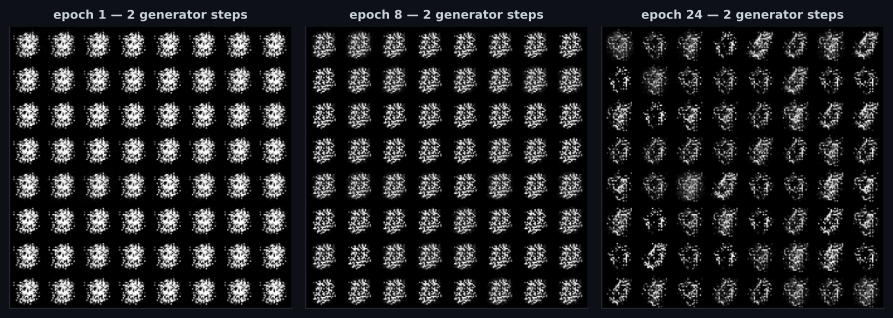
Mode collapse, measured: the default configuration put 79.6% of 2,000 samples on one digit; the best put 40.1% on one and produced 5 of 10 classes.
Which knob actually moved coverage — the ratio of generator to discriminator updates, not the discriminator’s learning rate.
Why a sample grid is not evidence, and what to compute instead.
The tricks that are load-bearing rather than folklore: one-sided label smoothing, LeakyReLU, separate optimisers, and freezing the discriminator at the right moment.

The game

Two networks, opposite objectives, one shared batch of data:

\min_G \max_D \; \mathbb{E}_{x \sim p_{\text{data}}}\big[\log D(x)\big] + \mathbb{E}_{z \sim p_z}\big[\log\big(1 - D(G(z))\big)\big]

The discriminator maximises its ability to separate real from fake; the generator minimises it. The equilibrium is where $D$ outputs 0.5 everywhere because the two distributions match — at which point the discriminator loss is $\log 2 = 0.6931$ and both accuracies sit at 0.5.

diagram Diagram mermaid

  flowchart LR
  Z["z ~ N(0, I)"] --> G["generator"]
  G --> F["fake images"]
  X["real images"] --> D["discriminator"]
  F --> D
  D --> R["real / fake probability"]
  R -->|"labels: real 0.9, fake 0"| DL["train D"]
  R -->|"labels: fakes called real
D frozen"| GL["train G"]
  DL -.->|"D acc real 0.9863
D acc fake 0.9999"| B["is the game balanced?"]
  GL -.->|"KL 6.0163 from uniform"| M["did it cover the data?"]

Note what is missing from that diagram: any path from a generated image to a measure of how good it is. The generator’s gradient comes entirely from the discriminator’s current opinion, and that opinion is a moving target.

Building it in Keras

Three models: the generator, the discriminator, and a combined model that stacks them so the generator can be trained through a frozen discriminator.

The three models

generator = keras.Sequential([
    keras.layers.Input((LATENT,)),
    keras.layers.Dense(128), keras.layers.LeakyReLU(negative_slope=0.2),
    keras.layers.Dense(256), keras.layers.LeakyReLU(negative_slope=0.2),
    keras.layers.Dense(784, activation="sigmoid"),      # pixels in [0, 1]
])
 
discriminator.compile(keras.optimizers.Adam(2e-4), "binary_crossentropy")
 
discriminator.trainable = False          # frozen while the combined model is built
combined_input = keras.layers.Input((LATENT,))
combined = keras.Model(combined_input, discriminator(generator(combined_input)))
combined.compile(keras.optimizers.Adam(2e-4), "binary_crossentropy")

Nearly every GAN tutorial written for Keras 2 ends that block with discriminator.trainable = True, on the theory that trainable is captured at compile time so the combined model keeps a permanently frozen copy. That was true then. It is not true in Keras 3, and the difference is not cosmetic — it silently trains the discriminator to agree that fakes are real.

Measured on Keras 3.15, building the combined model with the discriminator frozen and then setting the flag back:

Pattern	`combined.trainable_weights`	Largest discriminator weight change after 20 generator steps
Freeze, compile, set back to `True`	8 (the generator has 4)	0.01170799
Freeze, compile, leave frozen	4	0.00000000
Toggle around each generator step	4 during the step	0.00000000

The first row is the bug. The generator’s target is “call my fakes real”, so a trainable discriminator inside that step is dragged towards exactly the opinion it exists to oppose. The working pattern toggles the flag around the call:

python

def generator_step(combined, discriminator, noise):
    """Train the generator with the discriminator genuinely frozen."""
    discriminator.trainable = False
    loss = combined.train_on_batch(noise, np.ones((len(noise), 1), "float32"))
    discriminator.trainable = True      # so D can still train on its own batches
    return float(loss)

This page’s first run had the bug. Every number below comes from the corrected run, and the difference it made is reported at the end of this section.

LeakyReLU rather than ReLU is also load-bearing. A dead ReLU in the discriminator gives the generator zero gradient in that direction, and the generator has no other source of learning signal.

One step of the game

fake = generator.predict(noise, verbose=0)
 
# One-sided label smoothing: real labels at 0.9, fake labels left at 0.
d_real = discriminator.train_on_batch(batch, np.full((len(batch), 1), 0.9))
d_fake = discriminator.train_on_batch(fake, np.zeros((len(fake), 1)))
 
# The generator wants the discriminator to call its fakes real - with D frozen.
g_loss = generator_step(combined, discriminator, noise)

Label smoothing on the real side stops the discriminator becoming perfectly confident, which would flatten the gradient the generator depends on. It also has a measurement consequence, described below.

Reading the curves

Two panels covering four configurations. Left: generator loss rising over 24 epochs in every configuration, from 6.63 for the default down to 2.86 for the most heavily regularised one. Right: discriminator accuracy on fake batches, which climbs above 0.98 within two epochs in all four configurations and stays there, far above the dashed equilibrium line at 0.5. — A generator loss that rises for 24 straight epochs is a generator losing. The right panel says why: the discriminator identifies essentially every fake in every configuration — the best case still ends at 0.9966 against the 0.5 that equilibrium requires. Weakening the discriminator (lower learning rate, heavier dropout) narrowed the gap but never closed it, which is what makes GAN training different in kind from ordinary supervised training.

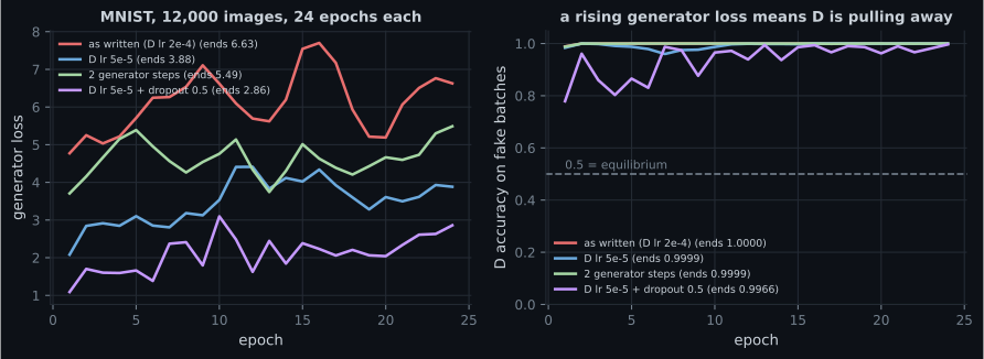
The best configuration by coverage, epoch by epoch:

Epoch	D loss	G loss	D accuracy on real	D accuracy on fake
1	0.2267	3.7070	0.9693	0.9879
2	0.2178	4.1576	0.9672	0.9999
23	0.1945	5.3003	0.9820	0.9999
24	0.1885	5.4879	0.9863	0.9999

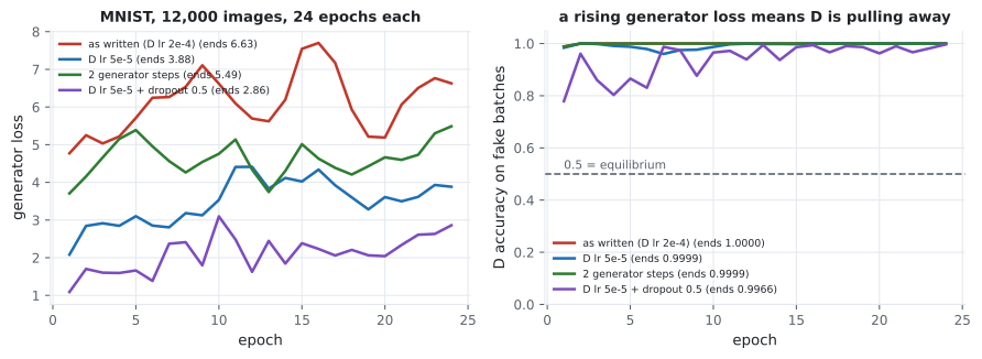
Every column points the same way. The discriminator loss falls towards zero rather than rising towards $\log 2 = 0.6931$ ; the generator loss climbs from 3.7070 to 5.4879; the discriminator catches 99.99% of fakes from epoch 2 onward. This is the too-strong discriminator failure, and it is not a subtle one.

Why it happens here is structural rather than accidental: the loop trains the discriminator twice per step — once on a real batch, once on a fake batch — against one generator update. That is what nearly every GAN tutorial does, so “as written” is a biased starting point, not a neutral one.

The balance sweep

Four ways of handing capacity back to the generator, each trained for 24 epochs:

Configuration	Classes	KL from uniform	Judge confidence	D accuracy on fake (last epoch)	Time
As written (D lr 2e-4)	2	14.4616	0.5520	1.0000	402s
D lr 5e-5	2	14.4384	0.5555	0.9999	461s
2 generator steps	5	6.0163	0.5798	0.9999	431s
D lr 5e-5 + dropout 0.5	2	14.4149	0.6709	0.9966	374s

Three things fall out of that table, and only the first was expected:

Doubling the generator’s updates more than doubled coverage — 2 classes to 5, KL 14.4616 to 6.0163. The update ratio is the knob that mattered.
Lowering the discriminator’s learning rate did essentially nothing (14.4616 → 14.4384). A slower discriminator is still a winning discriminator; it just gets there later.
The configuration with the best judge confidence had the worst coverage. Heavier dropout plus a slower discriminator gave the sharpest-looking samples (0.6709) and the lowest fake accuracy (0.9966) while still producing only 2 classes. Optimising the metric that is easy to look at would have selected exactly the wrong run.

The first version of this experiment reported discriminator accuracy on real batches as exactly 0.0000 at every epoch, which is impossible for a network that was plainly learning. The cause was mine: real labels are smoothed to 0.9, and Keras’s metrics=["accuracy"] compares the rounded prediction with y_true, so 0.9 matches neither 0 nor 1 and the metric reads zero forever. The fix is a metric that ignores the label and reports the decision:

python

def called_real(y_true, y_pred):
    del y_true                       # the smoothed label is not the question
    return tf.reduce_mean(tf.cast(y_pred > 0.5, "float32"))

With that in place, accuracy on real reads 0.9693 rising to 0.9863 across the best run. A metric that reports a constant is a broken metric, not a finding.

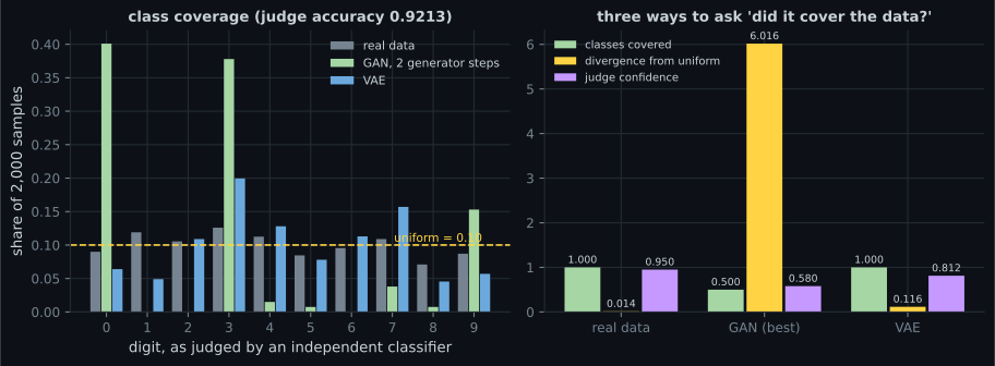
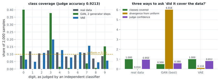
Mode collapse, measured

A grid of samples cannot tell you what a model never produces. So the samples were handed to a separate MNIST classifier — trained to 0.9213 validation accuracy, never shown a generated image — and the distribution of its predictions is the measurement.

figure 2,000 samples per model, judged by an independent classifier matplotlib

Even the best configuration puts 40.1% of its samples on the digit 0 and 37.8% on the digit 3, leaving 1, 2 and 6 entirely absent. Its KL from uniform coverage is 6.0163, against 0.0139 for real data and 0.1161 for the VAE. The right panel adds the part that surprised me: judge confidence on GAN samples is 0.5798, well below the VAE's 0.8121 — so the lost coverage did not buy sharpness.

Digit	0	1	2	3	4	5	6	7	8	9
Real	0.090	0.119	0.105	0.126	0.113	0.085	0.096	0.109	0.071	0.087
GAN, best	0.401	0.000	0.000	0.378	0.015	0.007	0.000	0.038	0.007	0.153
GAN, default	0.000	0.000	0.000	0.203	0.000	0.000	0.000	0.000	0.796	0.000
VAE	0.064	0.049	0.109	0.200	0.128	0.078	0.113	0.157	0.045	0.057

Mode collapse is those zeros. The generator found a small region of output space the discriminator was weakest on and had no reason to leave — nothing in the objective rewards diversity. Note that the default configuration and the best one collapsed onto different digits (8 versus 0 and 3), which is the tell that the collapsed mode is an accident of the run rather than a property of the data. And the generator loss says none of this: 5.4879 at the last epoch is a number with no interpretation.

Three uncurated 8 by 8 grids of generated images at epochs 1, 8 and 24 from the best configuration. Epoch 1 is unstructured noise with faint bright blobs, epoch 8 shows stroke-like shapes with repeated structure, and epoch 24 shows digit-like forms, most of them variations of a 0 or a 3. — These are the first 64 samples from a fixed noise batch, not a selection. The progress from epoch 1 to 24 is real, and so is the repetition: by epoch 24 most cells hold a variation of a 0 or a 3. This is what a KL of 6.0163 looks like when you plot it instead of computing it — and why the computed number is the honest way to report a GAN.

Why the VAE won here, and what that means

It would be easy to call the GAN sharper and quietly not measure it. The numbers say otherwise on this budget: two dense layers per network, latent 32, 24 epochs, 12,000 images, CPU only, across four configurations. Three conclusions worth keeping:

GAN sharpness is not free. The results people remember come from convolutional architectures (DCGAN and later), far longer training, and real hyperparameter search. A small dense GAN on a CPU is more likely to collapse than to sharpen.
At small scale the VAE is the more robust choice. It has an actual loss function, it converged without babysitting or a sweep, and it covered all ten classes at KL 0.1161 — against the best of four GAN runs at 6.0163.
Neither model’s loss revealed any of this. The coverage measurement did, and it cost one small classifier.

That third point generalises well past GANs, and the evaluation page turns it into three metrics that apply to any generative model.

Stabilising the game

The techniques below have a mechanism behind them, which is why they are here and the rest of the folklore is not:

One-sided label smoothing (real → 0.9). Keeps the discriminator from saturating.
LeakyReLU in both networks. A dead unit is a dead gradient path for the generator.
Separate Adam optimisers — here both at 2e-4, with beta_1 near 0.5 in published DCGAN work. The point is that the two networks must not share optimiser state.
Train D on real and fake in separate batches. Mixing them in one batch interacts badly with batch normalisation, since the batch statistics then straddle both distributions.
Count the updates. Two discriminator updates per generator update is the default in most tutorials, and moving to two generator updates was the only change here that improved coverage (KL 14.4616 → 6.0163).
Watch accuracy on fake batches, not the loss. All four runs pinned above 0.9966, which is the signature of a starved generator. Below roughly 0.5 the discriminator has instead stopped being informative.

If fake accuracy pins near 1.0 and the generator loss climbs for many epochs — 3.7070 to 5.4879 here — the run is not going to recover on its own. Change the balance and restart rather than waiting it out.

sketch The minimax game p5.js

Drag inside either bar to set how well the discriminator separates real from fake. The panel reports both losses and where the game sits relative to equilibrium.

sketch The measured table, ranked p5.js

Click a column to rank every row by it. The bars are that column's values and the highest and lowest are computed from the numbers, not written in.

Pitfalls

Judging a GAN by a sample grid. The grid cannot show the digits a model never produces. The classifier could: KL 6.0163 for the best run and 14.4616 for the default, against 0.0139 for real data.
Trusting metrics=["accuracy"] with smoothed labels. It reported 0.0000 at every epoch here, because 0.9 never equals a rounded prediction.
Reading the generator loss as quality. It rose every epoch, 3.7070 to 5.4879, in the run that covered the most classes.
Tuning only the discriminator’s learning rate. Dropping it from 2e-4 to 5e-5 moved coverage from KL 14.4616 to 14.4384 — nothing. The update ratio was the knob that worked.
Selecting a run by how sharp the samples look. The best judge confidence (0.6709) belonged to a run that produced 2 of 10 classes.
Copying the Keras 2 trainable idiom into Keras 3. Freeze, compile, unfreeze leaves 8 trainable tensors in the combined model and moved the discriminator’s weights 0.01170799 in 20 generator steps. Toggle the flag around each generator step instead.
Assuming GANs beat VAEs because the literature says so. On this budget the VAE won on coverage (10 classes against 5) and on judge confidence (0.8121 against 0.5798).
Comparing GAN losses across runs. They are not comparable — the scale depends on the discriminator’s current strength, which differs in every run.

Recap

A GAN replaces the reconstruction loss with a learned discriminator, so no loss measures sample quality any more.
Equilibrium is discriminator loss $\log 2 = 0.6931$ with both accuracies at 0.5. No configuration came close: discriminator loss fell to 0.1885 and fake accuracy pinned at 0.9999.
The default loop trains the discriminator twice per generator update. Reversing that ratio was the only change that improved coverage: 2 classes → 5, KL 14.4616 → 6.0163.
Lowering the discriminator’s learning rate changed nothing (14.4384), and the run with the sharpest samples had the worst coverage.
Both collapsed runs picked different digits, so the surviving mode is an artefact of the run.
The VAE on identical data covered 10 classes at KL 0.1161 with higher judge confidence — the usual sharpness-for-coverage trade did not appear at this scale.
The only reliable diagnostics were external: an independent classifier’s class distribution and confidence.

The measurements this page leaned on — coverage, an independent judge, and distance between distributions in feature space — deserve their own treatment, including how each one can be gamed: Evaluating Generative Models (FID, Coverage and Memorisation).

pch.quizTag pch.quizDefaultTitle

A GAN's generator loss rises steadily from 3.7070 to 5.4879 over 24 epochs. What does that mean?

pch.quizShowAnswer

B — The generator is losing — the discriminator is pulling away, which the fake-batch accuracy confirms at 0.9999 — The absolute value of a GAN loss means little, but its direction against a strengthening opponent does: a generator that cannot keep up sees its loss climb.
Every configuration in the sweep ended with discriminator accuracy on fake batches at 0.9966 or above. What does that indicate?

pch.quizShowAnswer

B — The generators were starved — a discriminator that catches essentially every fake gives almost no usable gradient, and equilibrium would be 0.5 — It is the signature of the too-strong-discriminator failure, and it is why the default loop's 2:1 update ratio in the discriminator's favour matters so much.
Lowering the discriminator's learning rate from 2e-4 to 5e-5 moved coverage KL from 14.4616 to 14.4384, while doubling the generator's updates moved it to 6.0163. What is the lesson?

pch.quizShowAnswer

B — The ratio of generator to discriminator updates was the effective knob here; a slower discriminator still wins, it just arrives later — Both changes weaken the discriminator in some sense, but only one changes how much learning signal the generator actually receives per epoch.
Why train an independent classifier just to score the samples?

pch.quizShowAnswer

B — Because neither GAN loss can detect mode collapse — the classifier's prediction distribution showed 5 of 10 classes covered at KL 6.0163 for the best run, and 2 classes at 14.4616 for the default — The judge never sees a generated image during its own training, so its class distribution over samples is an outside measurement rather than part of the game.
Keras reported discriminator accuracy on real batches as 0.0000 at every epoch. What was wrong?

pch.quizShowAnswer

B — The real labels were smoothed to 0.9, and binary accuracy compares the rounded prediction against y_true, so 0.9 matches neither 0 nor 1 — A metric that returns a constant is broken. Replacing it with a function that reports the share of the batch called real gave 0.9693 rising to 0.9863.
The VAE covered 10 classes at KL 0.1161 while the best of four GAN runs covered 5 at KL 6.0163, and the judge was more confident about VAE samples. What is the right conclusion?

pch.quizShowAnswer

B — At this scale — dense layers, 24 epochs, CPU — the GAN collapsed rather than sharpened; GAN sharpness results come from convolutional architectures with far more training, so the claim should not be assumed on a small budget — The measurement is specific to this budget, and saying so is more useful than repeating a claim this run did not reproduce.

🧪 Try It Yourself

pch.coffeeTagline

pch.coffeeCta

pch.feedbackHeading

pch.feedbackSubheading