Linearization and Multivariate Taylor Series

Everything in this chapter has been building one object without saying so. The gradient is a $1 \times D$ row; the Hessian is a $D \times D$ matrix; §5.7’s Remark mentioned a $D \times D \times D$ tensor and moved on. §5.8 finally says what they are: consecutive terms of a single series, each one a tensor of one higher order, each contracted against one more copy of the same displacement vector.

The section starts with the humblest possible use of the gradient and ends with a polynomial reproduced exactly.

What you’ll learn

• Equation 5.148, linearization — the one-line formula behind tangent planes, Gauss–Newton, delta-method error propagation, and every “assume it’s locally linear” argument you will ever read.
• Definition 5.7 and Equation 5.151: the multivariate Taylor series, and what $\boldsymbol{\delta}^k$ means when $\boldsymbol{\delta}$ is a vector.
• Definition 5.8: the Taylor polynomial $T_n$, and the fact that truncating a series is a local promise, measured.
• Equations 5.153 to 5.155: outer products, why order-$k$ derivatives are order-$k$ tensors, and the three einsum calls the book puts in its margin.
• Equations 5.156 to 5.160 written out for $k = 0, 1, 2, 3$, including why $\operatorname{tr}(H\boldsymbol{\delta}\boldsymbol{\delta}^\top)$ and $\boldsymbol{\delta}^\top H \boldsymbol{\delta}$ are the same number.
• Example 5.15 end to end: $f = x^2 + 2xy + y^3$ at $(1, 2)$, every equation from 5.161 to 5.180 reproduced and checked, including the claim that $T_3$ is $f$ — verified over a grid, not at a point.
• The two reasons nobody goes past second order: the term count, and the fact that on a fixed window a higher-order model can be worse.
• The Laplace approximation, which is a second-order Taylor expansion of a log-density wearing a different hat.

Intuition: three ways to answer “what does f look like near here?”

Someone asks you to describe a hillside at the spot you are standing.

The zeroth-order answer is a number: “the elevation here is 340 m.” Useless for walking, but it is right at one point.

The first-order answer adds a direction and a rate: “340 m, sloping up at 12% toward the north-east.” That is Equation 5.148, and it is a plane — the tangent plane. It is right at the point and it gets the slope right, so for small steps it is very good and for large steps it is a plane pretending to be a hill.

The second-order answer adds how the slope changes: “…and it curves away sharply to the left, gently ahead.” That is a quadratic bowl or saddle glued to the point, which is the Hessian’s job.

Each answer costs more to compute and each is only better near the point. Push far enough out and the extra terms turn on you: measured below, at radius 3.2 the quadratic model’s error is five times the constant model’s. That is not a bug; it is what “asymptotic” means.

diagram Diagram mermaid

  flowchart LR
  D["delta = x - x0
the displacement"] --> K0
  subgraph terms["Eq 5.156 to 5.160: one term per order"]
    K0["k=0: f(x0)
a scalar"]
    K1["k=1: grad f . delta
1 x D contracted once"]
    K2["k=2: delta' H delta / 2
D x D contracted twice"]
    K3["k=3: D3 f . delta^3 / 6
D x D x D contracted 3x"]
  end
  K0 --> T0["T0: the value"]
  K1 --> T1["T1: the tangent plane
Eq 5.148"]
  K2 --> T2["T2: plus curvature"]
  K3 --> T3["T3, Eq 5.152"]
  T3 --> EX["for a cubic f, T3 = f exactly
Eq 5.180c"]
  K2 --> COST["D^k entries at order k:
1e12 at D = 1e6, k = 2"]
  COST --> STOP["which is where practice stops"]

The math

Equation 5.148: linearization

The plainest use of a gradient:

$$f(\mathbf{x}) \approx f(\mathbf{x}_0) + (\nabla_{\mathbf{x}}f)(\mathbf{x}_0)(\mathbf{x} - \mathbf{x}_0) \tag{5.148}$$

Note the shapes, which are the reason §5.2 insisted the gradient be a row: $(\nabla_\mathbf{x}f)(\mathbf{x}_0)$ is $1 \times D$, $(\mathbf{x} - \mathbf{x}_0)$ is $D \times 1$, and the product is the scalar you add to $f(\mathbf{x}_0)$. No transposes to remember.

The book’s Figure 5.12 shows the univariate case: a curve linearized at $x_0 = -2$, approximated by a straight line, “locally accurate, but the farther we move away from $x_0$ the worse the approximation gets.” Equation 5.148 is a truncation of something larger, and the rest of §5.8 is that something.

Definition 5.7: the multivariate Taylor series

For $f : \mathbb{R}^D \to \mathbb{R}$ smooth at $\mathbf{x}_0$, with $\boldsymbol{\delta} := \mathbf{x} - \mathbf{x}_0$:

$$f(\mathbf{x}) = \sum_{k=0}^{\infty} \frac{D_{\mathbf{x}}^k f(\mathbf{x}_0)}{k!}\,\boldsymbol{\delta}^k \tag{5.151}$$

where $D^k_\mathbf{x} f(\mathbf{x}_0)$ is the $k$-th total derivative of $f$ with respect to $\mathbf{x}$, evaluated at $\mathbf{x}_0$.

Definition 5.8: the Taylor polynomial

$$T_n(\mathbf{x}) = \sum_{k=0}^{n} \frac{D_{\mathbf{x}}^k f(\mathbf{x}_0)}{k!}\,\boldsymbol{\delta}^k \tag{5.152}$$

the first $n+1$ terms of the series. Equation 5.148 is exactly $T_1$.

What delta-to-the-k means

The book flags its own notation as “slightly sloppy”: $\boldsymbol{\delta}^k$ is not defined for a vector when $k > 1$. Both $D^k_\mathbf{x}f$ and $\boldsymbol{\delta}^k$ are $k$-th order tensors — $k$-dimensional arrays — and $\boldsymbol{\delta}^k$ is the $k$-fold outer product $\otimes$ of $\boldsymbol{\delta}$ with itself:

$$\boldsymbol{\delta}^2 := \boldsymbol{\delta} \otimes \boldsymbol{\delta} = \boldsymbol{\delta}\boldsymbol{\delta}^\top, \qquad \boldsymbol{\delta}^2[i, j] = \delta[i]\,\delta[j] \tag{5.153}$$ $$\boldsymbol{\delta}^3 := \boldsymbol{\delta} \otimes \boldsymbol{\delta} \otimes \boldsymbol{\delta}, \qquad \boldsymbol{\delta}^3[i, j, k] = \delta[i]\,\delta[j]\,\delta[k] \tag{5.154}$$

Each outer product raises the dimensionality of the array by one, which is what the book’s Figure 5.13 draws: a vector in $\mathbb{R}^4$, then a $4 \times 4$ matrix, then a $4 \times 4 \times 4$ cube. Then the general term is a full contraction — every index of the derivative tensor paired with one copy of $\boldsymbol{\delta}$:

$$D^k_\mathbf{x}f(\mathbf{x}_0)\boldsymbol{\delta}^k = \sum_{i_1=1}^{D}\cdots\sum_{i_k=1}^{D} D^k_\mathbf{x}f(\mathbf{x}_0)[i_1, \ldots, i_k]\,\delta[i_1]\cdots\delta[i_k] \tag{5.155}$$

which is a $k$-th order polynomial in the components of $\boldsymbol{\delta}$.

Equations 5.156 to 5.160: the first four terms

$$k = 0: \quad D^0_\mathbf{x}f(\mathbf{x}_0)\boldsymbol{\delta}^0 = f(\mathbf{x}_0) \in \mathbb{R} \tag{5.156}$$ $$k = 1: \quad D^1_\mathbf{x}f(\mathbf{x}_0)\boldsymbol{\delta}^1 = \underbrace{\nabla_\mathbf{x}f(\mathbf{x}_0)}_{1 \times D}\underbrace{\boldsymbol{\delta}}_{D \times 1} = \sum_{i=1}^{D}\nabla_\mathbf{x}f(\mathbf{x}_0)[i]\,\delta[i] \tag{5.157}$$ $$k = 2: \quad D^2_\mathbf{x}f(\mathbf{x}_0)\boldsymbol{\delta}^2 = \operatorname{tr}\bigl(\underbrace{H(\mathbf{x}_0)}_{D \times D}\underbrace{\boldsymbol{\delta}}_{D \times 1}\underbrace{\boldsymbol{\delta}^\top}_{1 \times D}\bigr) = \boldsymbol{\delta}^\top H(\mathbf{x}_0)\boldsymbol{\delta} \tag{5.158}$$ $$= \sum_{i=1}^{D}\sum_{j=1}^{D} H[i,j]\,\delta[i]\,\delta[j] \tag{5.159}$$ $$k = 3: \quad D^3_\mathbf{x}f(\mathbf{x}_0)\boldsymbol{\delta}^3 = \sum_{i=1}^{D}\sum_{j=1}^{D}\sum_{k=1}^{D} D^3_\mathbf{x}f(\mathbf{x}_0)[i,j,k]\,\delta[i]\,\delta[j]\,\delta[k] \tag{5.160}$$

Two things worth pausing on.

Equation 5.158’s two forms are the same number. $\boldsymbol{\delta}\boldsymbol{\delta}^\top$ is a $D \times D$ rank-one matrix; multiplying by $H$ and taking the trace contracts both indices, and that is exactly what $\boldsymbol{\delta}^\top H \boldsymbol{\delta}$ does. Verified below to $0.0\text{e-}00$ at four displacements. The trace form is the one that generalises to arbitrary $k$; the quadratic form is the one you should actually compute, since it never builds the $D \times D$ intermediate.

The margin of page 167 gives the code. The book puts three NumPy calls beside these equations, and they are the cleanest statement of the pattern:

$$\texttt{np.einsum('i,i', Df1, d)}, \quad \texttt{np.einsum('ij,i,j', Df2, d, d)}, \quad \texttt{np.einsum('ijk,i,j,k', Df3, d, d, d)}$$

One index letter per tensor order, one d per copy of $\boldsymbol{\delta}$. The pattern for order $k$ writes itself.

Where the factorials come from

Equation 5.151 divides the $k$-th term by $k!$, and Equation 5.159’s double sum runs over all ordered pairs $(i, j)$ — so the cross term $H[1,2]\delta_1\delta_2$ is counted twice, once as $(1,2)$ and once as $(2,1)$. That is why Equation 5.173c’s expansion has $2(x-1)(y-2)$ with a factor of 2 while the squared terms do not, and why the $\tfrac{1}{2}$ out front does not simply cancel. Getting this wrong by a factor of two is the single most common error in hand-expanding a multivariate Taylor series.

Worked example by hand

The book’s Example 5.15, in full. Expand

$$f(x, y) = x^2 + 2xy + y^3 \tag{5.161}$$

at $(x_0, y_0) = (1, 2)$.

Predict the answer first. $f$ is a polynomial of degree 3, and a Taylor expansion is a linear combination of polynomials. So there is no way a term of fourth order or higher can appear, and the first four terms of Equation 5.151 ought to reproduce $f$ exactly. The book makes this prediction before computing anything, and it is a good habit: it tells you what a correct answer looks like.

Order 0.

$$f(1, 2) = 1 + 4 + 8 = 13 \tag{5.162}$$

Order 1. Differentiate once in each variable:

$$\frac{\partial f}{\partial x} = 2x + 2y \implies \frac{\partial f}{\partial x}(1,2) = 2 + 4 = 6 \tag{5.163}$$ $$\frac{\partial f}{\partial y} = 2x + 3y^2 \implies \frac{\partial f}{\partial y}(1,2) = 2 + 12 = 14 \tag{5.164}$$

so

$$D^1_{x,y}f(1,2) = \nabla_{x,y}f(1,2) = \begin{bmatrix} 6 & 14 \end{bmatrix} \in \mathbb{R}^{1 \times 2} \tag{5.165}$$

and the first-order term is

$$\frac{D^1_{x,y}f(1,2)}{1!}\boldsymbol{\delta} = \begin{bmatrix} 6 & 14 \end{bmatrix}\begin{bmatrix} x - 1 \\ y - 2 \end{bmatrix} = 6(x-1) + 14(y-2) \tag{5.166}$$

Linear terms only, as promised.

Order 2. Four second partials:

$$\frac{\partial^2 f}{\partial x^2} = 2 \implies 2, \qquad \frac{\partial^2 f}{\partial y^2} = 6y \implies 12 \tag{5.167, 5.168}$$ $$\frac{\partial^2 f}{\partial y\,\partial x} = 2, \qquad \frac{\partial^2 f}{\partial x\,\partial y} = 2 \tag{5.169, 5.170}$$

The last two agree, which is Equation 5.146 doing its job. Collect:

$$H = \begin{bmatrix} 2 & 2 \\ 2 & 6y \end{bmatrix}, \qquad H(1,2) = \begin{bmatrix} 2 & 2 \\ 2 & 12 \end{bmatrix} \in \mathbb{R}^{2\times 2} \tag{5.171, 5.172}$$

and the second-order term is

$$\frac{D^2_{x,y}f(1,2)}{2!}\boldsymbol{\delta}^2 = \tfrac{1}{2}\boldsymbol{\delta}^\top H(1,2)\boldsymbol{\delta} \tag{5.173a}$$ $$= \tfrac{1}{2}\begin{bmatrix} x-1 & y-2 \end{bmatrix}\begin{bmatrix} 2 & 2 \\ 2 & 12 \end{bmatrix}\begin{bmatrix} x-1 \\ y-2 \end{bmatrix} \tag{5.173b}$$ $$= (x-1)^2 + 2(x-1)(y-2) + 6(y-2)^2 \tag{5.173c}$$

Multiply that out by hand to see where each coefficient comes from. The quadratic form is $2\delta_1^2 + 2\delta_1\delta_2 + 2\delta_2\delta_1 + 12\delta_2^2 = 2\delta_1^2 + 4\delta_1\delta_2 + 12\delta_2^2$; halve it and you get $\delta_1^2 + 2\delta_1\delta_2 + 6\delta_2^2$. The cross term kept its factor of 2 because the double sum counted it twice.

Order 3. The third derivative is a $2 \times 2 \times 2$ tensor, and the book writes it as two slices — the derivative of the Hessian with respect to each variable:

$$D^3_{x,y}f = \begin{bmatrix} \dfrac{\partial H}{\partial x} & \dfrac{\partial H}{\partial y} \end{bmatrix} \in \mathbb{R}^{2\times 2\times 2} \tag{5.174}$$

Look back at Equation 5.171. Three of its four entries are constants, so they differentiate to zero. The only surviving third derivative is

$$\frac{\partial^3 f}{\partial y^3} = 6 \implies \frac{\partial^3 f}{\partial y^3}(1,2) = 6 \tag{5.177}$$

giving

$$D^3_{x,y}f[:,:,1] = \begin{bmatrix} 0 & 0 \\ 0 & 0\end{bmatrix}, \qquad D^3_{x,y}f[:,:,2] = \begin{bmatrix} 0 & 0 \\ 0 & 6\end{bmatrix} \tag{5.178}$$

One nonzero number in eight slots. The third-order term is therefore

$$\frac{D^3_{x,y}f(1,2)}{3!}\boldsymbol{\delta}^3 = \frac{6}{6}(y-2)^3 = (y-2)^3 \tag{5.179}$$

Assemble.

$$f(\mathbf{x}) = 13 + 6(x-1) + 14(y-2) + (x-1)^2 + 6(y-2)^2 + 2(x-1)(y-2) + (y-2)^3 \tag{5.180c}$$

Order	Tensor	Shape	Nonzero entries	Contributes
0	$f(1,2)$	scalar	1	$13$
1	$\nabla f$	$1 \times 2$	2	$6(x-1) + 14(y-2)$
2	$H$	$2 \times 2$	4	$(x-1)^2 + 2(x-1)(y-2) + 6(y-2)^2$
3	$D^3 f$	$2 \times 2 \times 2$	1 of 8	$(y-2)^3$
$\ge 4$	—	—	0	nothing

Check it at a point far from the expansion. Take $(6, -4)$, which is $\boldsymbol{\delta} = (5, -6)$ away — nowhere near “local”:

$$13 + 6(5) + 14(-6) + 25 + 6(36) + 2(5)(-6) + (-6)^3 = 13 + 30 - 84 + 25 + 216 - 60 - 216 = -76$$

and $f(6,-4) = 36 + 2(6)(-4) + (-4)^3 = 36 - 48 - 64 = -76$. Exact, at a displacement of $\|\boldsymbol{\delta}\| = 7.81$, because a degree-3 polynomial has room for every term a cubic has. This is the one situation where “Taylor series” and “algebraic identity” mean the same thing.

See it move

Start with the picture the book’s Figure 5.12 draws — the univariate case, so there is nothing to hide behind:

fieldFigure 5.12's linearization, and the degrees above itTaylor polynomials, §5.1.1

T_0(x) = - 1.325444

degree 0 of 5|f − T| within ±0.5 3.99e-1on the whole window 2.7395local order h^1

a0 -1.325444a1 0.493151a2 0.662722a3 -0.082192a4 -0.055227a5 0.00411a6 0.001841a7 -0.000098

T_n(x0) = f(x0) 0.0e+0

1T_n(x) = sum_{k=0}^{n} f^(k)(x0)/k! * (x - x0)^k      # Eq 5.72 3coeffs = jet(f, x0, N)          # a_k = f^(k)(x0)/k!, by jet arithmetic4for n in 0..N:5    T_n = lambda x: sum(coeffs[k] * (x - x0)**k for k in range(n + 1))6    err = max(abs(f(x) - T_n(x)) for x in window)

degree0|f − T_n| near x03.99e-1on the whole window2.740

Degree 0: T_0 is the constant f(x0) = -1.325444 — a horizontal line touching f at exactly one point. error within ±0.5 of x0 is 3.99e-1.

Play‹›1/6⟲

Expanded at x0 = -2, exactly as the book's figure. T1 is Equation 5.148: a straight line, right at the point and drifting away from f everywhere else. Watch both error numbers as the degree climbs — the one measured near x0 falls every time, the one measured over the whole window does not.

fieldThe same construction on a function whose series has a radiusTaylor polynomials, §5.1.1

T_0(x) = 0.5

degree 0 of 5|f − T| within ±0.5 1.22e-1on the whole window 0.4975local order h^1

a0 0.5a1 0.25a2 0a3 -0.020833a4 0a5 0.002083a6 0a7 -0.000211

T_n(x0) = f(x0) 0.0e+0

1T_n(x) = sum_{k=0}^{n} f^(k)(x0)/k! * (x - x0)^k      # Eq 5.72 3coeffs = jet(f, x0, N)          # a_k = f^(k)(x0)/k!, by jet arithmetic4for n in 0..N:5    T_n = lambda x: sum(coeffs[k] * (x - x0)**k for k in range(n + 1))6    err = max(abs(f(x) - T_n(x)) for x in window)

degree0|f − T_n| near x01.22e-1on the whole window0.4975

Degree 0: T_0 is the constant f(x0) = 0.5 — a horizontal line touching f at exactly one point. error within ±0.5 of x0 is 1.22e-1.

Play‹›1/6⟲

A sigmoid expanded at 0. Every added degree improves the fit near the origin and makes the tails worse, and the lab reports both. This is the honest version of 'higher order is better': it is a statement about a shrinking neighbourhood, not about the plot you are looking at.

sketch T0, T1, T2 on a surface p5.js Pause Restart

Drag the expansion point around the surface and the radius of the disc the error is measured on. Grey contours are f; coloured contours are the model. The three error numbers are maxima over the disc, so the moment the quadratic model stops helping is a number on the screen rather than a judgement call.

sketch Figure 5.13: outer products grow an index per term p5.js Pause Restart

The book's Figure 5.13 as a live count. Slide D and k and watch delta-to-the-k gain a dimension: a vector, then a matrix, then a cube. The entry count is D to the k, the distinct count after Equation 5.146's symmetry is the binomial C(D+k-1, k), and the gap between those two and the memory line is the whole reason Definition 5.8 stops at n = 2 in practice.

sketch The Laplace approximation is Equation 5.152 at n = 2 p5.js Pause Restart

Expand the LOG of a density to second order at its mode and exponentiate: a parabola becomes a Gaussian. Drag the expansion point off the mode and watch the approximation stop being a density at all — the curvature goes the wrong way and there is no Gaussian to be had.

From scratch

Example 5.15, every equation checked — including the three einsum calls from the book’s margin and the claim that $T_3$ is $f$:

example_5_15.py

import numpy as np
 
# Eq 5.161, the function Example 5.15 expands.
f = lambda x, y: x ** 2 + 2 * x * y + y ** 3
x0, y0 = 1.0, 2.0
 
# The derivatives, by hand. Each one is a line of algebra, written out on the page.
fx = lambda x, y: 2 * x + 2 * y            # Eq 5.163
fy = lambda x, y: 2 * x + 3 * y ** 2       # Eq 5.164
fxx = lambda x, y: 2.0                     # Eq 5.167
fyy = lambda x, y: 6 * y                   # Eq 5.168
fxy = lambda x, y: 2.0                     # Eq 5.169 and 5.170, equal by Eq 5.146
 
print(f"f(x, y) = x^2 + 2xy + y^3   expanded at (x0, y0) = ({x0:.0f}, {y0:.0f})")
print()
print(f"  Eq 5.162   f(1, 2)                = {f(x0, y0):.0f}")
print(f"  Eq 5.163   df/dx  = 2x + 2y       = {fx(x0, y0):.0f}")
print(f"  Eq 5.164   df/dy  = 2x + 3y^2     = {fy(x0, y0):.0f}")
D1 = np.array([[fx(x0, y0), fy(x0, y0)]])                       # Eq 5.165
print(f"  Eq 5.165   D1 = {D1.tolist()}, shape {D1.shape} -- a ROW vector, R^(1x2)")
print(f"  Eq 5.167   d2f/dx2  = 2           = {fxx(x0, y0):.0f}")
print(f"  Eq 5.168   d2f/dy2  = 6y          = {fyy(x0, y0):.0f}")
print(f"  Eq 5.169   d2f/dydx = 2           = {fxy(x0, y0):.0f}")
print(f"  Eq 5.170   d2f/dxdy = 2           = {fxy(x0, y0):.0f}   equal, by Eq 5.146")
H = np.array([[fxx(x0, y0), fxy(x0, y0)],
              [fxy(x0, y0), fyy(x0, y0)]])                      # Eq 5.172
print(f"  Eq 5.172   H(1, 2) = {H.tolist()}")
 
# The third derivative is a 2 x 2 x 2 tensor. Only d3f/dy3 = 6 survives, because
# every other second partial in Eq 5.171 is a constant.
D3 = np.zeros((2, 2, 2))
D3[1, 1, 1] = 6.0                                               # Eq 5.177
print(f"  Eq 5.177   d3f/dy3 = 6")
print(f"  Eq 5.178   D3[:, :, 1] = {D3[:, :, 0].tolist()}")
print(f"             D3[:, :, 2] = {D3[:, :, 1].tolist()}")
print(f"             {D3.size} entries, {int((D3 != 0).sum())} of them nonzero")
 
print()
print("The four terms, in the three notations the book uses")
print("  (the margin of p.167 gives exactly these einsum calls)")
for pt in ((2.0, 3.0), (1.5, 0.5), (-1.0, 4.0), (6.0, -4.0)):
    d = np.array([pt[0] - x0, pt[1] - y0])                      # delta, Def 5.7
    k0 = f(x0, y0)                                              # Eq 5.156
    k1 = np.einsum("i,i", D1.ravel(), d)                        # Eq 5.157
    k2_trace = np.trace(H @ np.outer(d, d))                     # Eq 5.158, form 1
    k2_quad = d @ H @ d                                         # Eq 5.158, form 2
    k2_sum = np.einsum("ij,i,j", H, d, d)                       # Eq 5.159
    k3 = np.einsum("ijk,i,j,k", D3, d, d, d)                    # Eq 5.160
    T3 = k0 + k1 / 1 + k2_quad / 2 + k3 / 6                     # Eq 5.180a
    print(f"  x = ({pt[0]:>5.1f}, {pt[1]:>5.1f})   delta = {d}")
    print(f"    k=0 {k0:>10.4f}    k=1 {k1:>10.4f}    k=2 {k2_quad:>10.4f}    k=3 {k3:>10.4f}")
    print(f"    tr(H d d^T) {k2_trace:>12.8f}  =  d^T H d {k2_quad:>12.8f}"
          f"  =  einsum {k2_sum:>12.8f}")
    print(f"    T3 = {T3:>12.6f}    f(x) = {f(*pt):>12.6f}    gap {abs(T3 - f(*pt)):.1e}")
 
print()
print("Eq 5.180c claims T3 IS f. Test it everywhere, not at one point.")
 
 
def T(n, X, Y):
    """The Taylor polynomial of degree n, Def 5.8, written out for this f."""
    dx, dy = X - x0, Y - y0
    out = np.full_like(X, f(x0, y0))
    if n >= 1:
        out = out + 6 * dx + 14 * dy
    if n >= 2:
        out = out + 0.5 * (2 * dx ** 2 + 2 * 2 * dx * dy + 12 * dy ** 2)
    if n >= 3:
        out = out + dy ** 3
    return out
 
 
gx, gy = np.meshgrid(np.linspace(-4, 6, 61), np.linspace(-4, 6, 61))
truth = f(gx, gy)
print(f"  over a 61 x 61 grid spanning [-4, 6] in both variables:")
print(f"    {'degree':>7}  {'max error':>13}  {'mean error':>12}")
for n in range(4):
    err = np.abs(truth - T(n, gx, gy))
    print(f"    T{n:<6}  {err.max():>13.4f}  {err.mean():>12.4f}")
print("  T3 is exact EVERYWHERE, not merely near (1, 2), because f is a cubic and a")
print("  degree-3 polynomial has room for every term a cubic has. Note also how")
print("  little T2 buys over T1 on this wide a grid: 216 against 225. Truncated")
print("  Taylor series are a LOCAL promise.")

output

f(x, y) = x^2 + 2xy + y^3   expanded at (x0, y0) = (1, 2)
 
  Eq 5.162   f(1, 2)                = 13
  Eq 5.163   df/dx  = 2x + 2y       = 6
  Eq 5.164   df/dy  = 2x + 3y^2     = 14
  Eq 5.165   D1 = [[6.0, 14.0]], shape (1, 2) -- a ROW vector, R^(1x2)
  Eq 5.167   d2f/dx2  = 2           = 2
  Eq 5.168   d2f/dy2  = 6y          = 12
  Eq 5.169   d2f/dydx = 2           = 2
  Eq 5.170   d2f/dxdy = 2           = 2   equal, by Eq 5.146
  Eq 5.172   H(1, 2) = [[2.0, 2.0], [2.0, 12.0]]
  Eq 5.177   d3f/dy3 = 6
  Eq 5.178   D3[:, :, 1] = [[0.0, 0.0], [0.0, 0.0]]
             D3[:, :, 2] = [[0.0, 0.0], [0.0, 6.0]]
             8 entries, 1 of them nonzero
 
The four terms, in the three notations the book uses
  (the margin of p.167 gives exactly these einsum calls)
  x = (  2.0,   3.0)   delta = [1. 1.]
    k=0    13.0000    k=1    20.0000    k=2    18.0000    k=3     6.0000
    tr(H d d^T)  18.00000000  =  d^T H d  18.00000000  =  einsum  18.00000000
    T3 =    43.000000    f(x) =    43.000000    gap 0.0e+00
  x = (  1.5,   0.5)   delta = [ 0.5 -1.5]
    k=0    13.0000    k=1   -18.0000    k=2    24.5000    k=3   -20.2500
    tr(H d d^T)  24.50000000  =  d^T H d  24.50000000  =  einsum  24.50000000
    T3 =     3.875000    f(x) =     3.875000    gap 0.0e+00
  x = ( -1.0,   4.0)   delta = [-2.  2.]
    k=0    13.0000    k=1    16.0000    k=2    40.0000    k=3    48.0000
    tr(H d d^T)  40.00000000  =  d^T H d  40.00000000  =  einsum  40.00000000
    T3 =    57.000000    f(x) =    57.000000    gap 0.0e+00
  x = (  6.0,  -4.0)   delta = [ 5. -6.]
    k=0    13.0000    k=1   -54.0000    k=2   362.0000    k=3 -1296.0000
    tr(H d d^T) 362.00000000  =  d^T H d 362.00000000  =  einsum 362.00000000
    T3 =   -76.000000    f(x) =   -76.000000    gap 0.0e+00
 
Eq 5.180c claims T3 IS f. Test it everywhere, not at one point.
  over a 61 x 61 grid spanning [-4, 6] in both variables:
     degree      max error    mean error
    T0            311.0000       48.1335
    T1            225.0000       40.4129
    T2            216.0000       40.4945
    T3              0.0000        0.0000
  T3 is exact EVERYWHERE, not merely near (1, 2), because f is a cubic and a
  degree-3 polynomial has room for every term a cubic has. Note also how
  little T2 buys over T1 on this wide a grid: 216 against 225. Truncated
  Taylor series are a LOCAL promise.

Now the two facts that decide how Taylor expansions are actually used:

taylor_in_practice.py

import math
 
import numpy as np
 
# A function that is NOT a polynomial, so no finite Taylor polynomial is exact.
g = lambda x, y: np.exp(-0.5 * (x ** 2 + y ** 2)) + 0.3 * np.sin(2 * x)
x0, y0 = 0.4, -0.3
 
 
def derivs(fn, x, y, h=1e-3):
    """Value, gradient and Hessian by central differences."""
    v = fn(x, y)
    dx = (fn(x + h, y) - fn(x - h, y)) / (2 * h)
    dy = (fn(x, y + h) - fn(x, y - h)) / (2 * h)
    dxx = (fn(x + h, y) - 2 * v + fn(x - h, y)) / h ** 2
    dyy = (fn(x, y + h) - 2 * v + fn(x, y - h)) / h ** 2
    dxy = (fn(x + h, y + h) - fn(x + h, y - h)
           - fn(x - h, y + h) + fn(x - h, y - h)) / (4 * h ** 2)
    return v, dx, dy, dxx, dxy, dyy
 
 
v, dx, dy, dxx, dxy, dyy = derivs(g, x0, y0)
th = np.linspace(0, 2 * np.pi, 720)
 
 
def models(rad):
    """T0, T1 and T2 evaluated on the circle of radius rad about (x0, y0)."""
    px, py = x0 + rad * np.cos(th), y0 + rad * np.sin(th)
    a, b = px - x0, py - y0
    t0 = np.full_like(px, v)
    t1 = t0 + dx * a + dy * b
    t2 = t1 + 0.5 * (dxx * a ** 2 + 2 * dxy * a * b + dyy * b ** 2)
    return g(px, py), t0, t1, t2
 
 
print("g(x, y) = exp(-(x^2 + y^2)/2) + 0.3 sin(2x)   expanded at (0.4, -0.3)")
print(f"  grad = [{dx:.6f} {dy:.6f}]")
print(f"  H    = [[{dxx:.6f} {dxy:.6f}], [{dxy:.6f} {dyy:.6f}]]")
print()
print("Error on the circle of radius r -- and whether more order is more accuracy")
print(f"  {'r':>6}  {'T0 max err':>11}  {'T1 max err':>11}  {'T2 max err':>11}"
      f"  {'T1/T0':>7}  {'T2/T1':>7}")
for rad in (0.05, 0.1, 0.2, 0.4, 0.8, 1.6, 3.2):
    tv, t0, t1, t2 = models(rad)
    e0 = np.abs(tv - t0).max()
    e1 = np.abs(tv - t1).max()
    e2 = np.abs(tv - t2).max()
    print(f"  {rad:>6.2f}  {e0:>11.6f}  {e1:>11.6f}  {e2:>11.6f}"
          f"  {e1 / e0:>7.3f}  {e2 / e1:>7.3f}")
print("  Read the two ratio columns. Close in, each order divides the error. Past")
print("  r = 1.6 the ratios cross 1 and the higher-order model is WORSE on that")
print("  ring -- at r = 3.2, T2's error of 7.77 is five times T0's 1.40. 'Higher")
print("  order is better' is a statement about a limit, not about a window.")
 
print()
print("The order itself, fitted rather than assumed (error should go like r^(n+1))")
rs = np.array([0.02, 0.04, 0.08])
for n, name in ((0, "T0"), (1, "T1"), (2, "T2")):
    es = []
    for rad in rs:
        tv, t0, t1, t2 = models(rad)
        model = (t0, t1, t2)[n]
        es.append(float(np.abs(tv - model).max()))
    slope = float(np.polyfit(np.log(rs), np.log(es), 1)[0])
    print(f"  {name}:  {es[0]:.3e}  {es[1]:.3e}  {es[2]:.3e}"
          f"   ->  slope {slope:.3f}   (expected {n + 1})")
 
print()
print("What Eq 5.151 costs at order k: the tensor D^k_x f has D^k entries")
print(f"  {'D':>11}  {'k=1':>13}  {'k=2 distinct':>16}  {'k=2 stored':>18}  {'k=3 distinct':>24}")
for D in (2, 10, 100, 1000, 1_000_000):
    print(f"  {D:>11,}  {D:>13,}  {math.comb(D + 1, 2):>16,}"
          f"  {D * D:>18,}  {math.comb(D + 2, 3):>24,}")
print("  Eq 5.146's symmetry cuts the k=2 count roughly in half -- C(D+1, 2) rather")
print("  than D^2 -- and it does not help at all with the exponent. At a million")
print("  parameters the Hessian is 1e12 numbers, 4 TB in float32, and the third-order")
print("  tensor is 1.7e17. That is why Def 5.8 is almost never used past n = 2.")
 
print()
print("Why Section 5.8 is in a machine-learning book: the Laplace approximation")
# An unnormalised skewed density. Its log is what gets expanded.
logp = lambda x: 2.5 * np.log(np.clip(x, 1e-12, None)) - 1.6 * x
# The mode, by golden-section search on log p. No optimiser import needed.
inv_phi = (np.sqrt(5) - 1) / 2
a, b = 0.05, 20.0
c, d = b - inv_phi * (b - a), a + inv_phi * (b - a)
while b - a > 1e-12:
    if logp(c) > logp(d):
        b, d = d, c
        c = b - inv_phi * (b - a)
    else:
        a, c = c, d
        d = a + inv_phi * (b - a)
mode = 0.5 * (a + b)
h = 1e-4
curv = (logp(mode + h) - 2 * logp(mode) + logp(mode - h)) / h ** 2
sigma2 = -1.0 / curv
print(f"  mode x*                       {mode:.6f}   (analytic 2.5/1.6 = {2.5 / 1.6:.6f})")
print(f"  d2 log p / dx2 at the mode    {curv:.6f}   (analytic -2.5/x*^2 = {-2.5 / mode ** 2:.6f})")
print(f"  the second-order expansion of log p is a PARABOLA, so exp of it is a")
print(f"  Gaussian: mean x* = {mode:.6f}, variance -1/H = {sigma2:.6f}")
 
# Compare the two densities on a fine grid; trapezoid is plenty here.
xs = np.linspace(-6, 40, 400001)
px = np.where(xs > 0, np.exp(logp(np.where(xs > 0, xs, 1.0))), 0.0)
px = px / np.trapezoid(px, xs)
qx = np.exp(-0.5 * (xs - mode) ** 2 / sigma2) / np.sqrt(2 * np.pi * sigma2)
tv_dist = 0.5 * np.trapezoid(np.abs(px - qx), xs)
below = np.trapezoid(qx[xs < 0], xs[xs < 0])
print(f"  total variation distance      {tv_dist:.6f}")
print(f"  Gaussian mass at x < 0        {below:.6f}")
print("  The last number is the honest limitation: p is supported on x > 0 and the")
print("  Laplace Gaussian is not, so it assigns real probability to impossible")
print("  values. A second-order expansion matches the mode and the curvature there;")
print("  it knows nothing about the support, the skew, or the tails.")

output

g(x, y) = exp(-(x^2 + y^2)/2) + 0.3 sin(2x)   expanded at (0.4, -0.3)
  grad = [0.065025 0.264749]
  H    = [[-1.602124 -0.105900], [-0.105900 -0.803072]]
 
Error on the circle of radius r -- and whether more order is more accuracy
       r   T0 max err   T1 max err   T2 max err    T1/T0    T2/T1
    0.05     0.014762     0.002034     0.000021    0.138    0.010
    0.10     0.031846     0.008178     0.000170    0.257    0.021
    0.20     0.073583     0.032926     0.001408    0.447    0.043
    0.40     0.190035     0.131281     0.013103    0.691    0.100
    0.80     0.519858     0.490258     0.139301    0.943    0.284
    1.60     1.197958     1.367102     1.355998    1.141    0.992
    3.20     1.396508     2.197040     7.772019    1.573    3.537
  Read the two ratio columns. Close in, each order divides the error. Past
  r = 1.6 the ratios cross 1 and the higher-order model is WORSE on that
  ring -- at r = 3.2, T2's error of 7.77 is five times T0's 1.40. 'Higher
  order is better' is a statement about a limit, not about a window.
 
The order itself, fitted rather than assumed (error should go like r^(n+1))
  T0:  5.632e-03  1.163e-02  2.473e-02   ->  slope 1.067   (expected 1)
  T1:  3.241e-04  1.300e-03  5.224e-03   ->  slope 2.005   (expected 2)
  T2:  1.313e-06  1.061e-05  8.629e-05   ->  slope 3.019   (expected 3)
 
What Eq 5.151 costs at order k: the tensor D^k_x f has D^k entries
            D            k=1      k=2 distinct          k=2 stored              k=3 distinct
            2              2                 3                   4                         4
           10             10                55                 100                       220
          100            100             5,050              10,000                   171,700
        1,000          1,000           500,500           1,000,000               167,167,000
    1,000,000      1,000,000   500,000,500,000   1,000,000,000,000   166,667,166,667,000,000
  Eq 5.146's symmetry cuts the k=2 count roughly in half -- C(D+1, 2) rather
  than D^2 -- and it does not help at all with the exponent. At a million
  parameters the Hessian is 1e12 numbers, 4 TB in float32, and the third-order
  tensor is 1.7e17. That is why Def 5.8 is almost never used past n = 2.
 
Why Section 5.8 is in a machine-learning book: the Laplace approximation
  mode x*                       1.562500   (analytic 2.5/1.6 = 1.562500)
  d2 log p / dx2 at the mode    -1.024000   (analytic -2.5/x*^2 = -1.024000)
  the second-order expansion of log p is a PARABOLA, so exp of it is a
  Gaussian: mean x* = 1.562500, variance -1/H = 0.976563
  total variation distance      0.165397
  Gaussian mass at x < 0        0.056911
  The last number is the honest limitation: p is supported on x > 0 and the
  Laplace Gaussian is not, so it assigns real probability to impossible
  values. A second-order expansion matches the mode and the curvature there;
  it knows nothing about the support, the skew, or the tails.

The T1/T0 and T2/T1 columns are the honest version of “higher order is better”. Close in they are $0.138$ and $0.010$ — each order divides the error by a lot. At $r = 1.6$ they are $1.141$ and $0.992$: the first-order model has become worse than the constant, and the second-order model has stopped helping. At $r = 3.2$, $T_2$‘s error is $7.77$ against $T_0$‘s $1.40$ — the most sophisticated model on the table is five times the worst one.

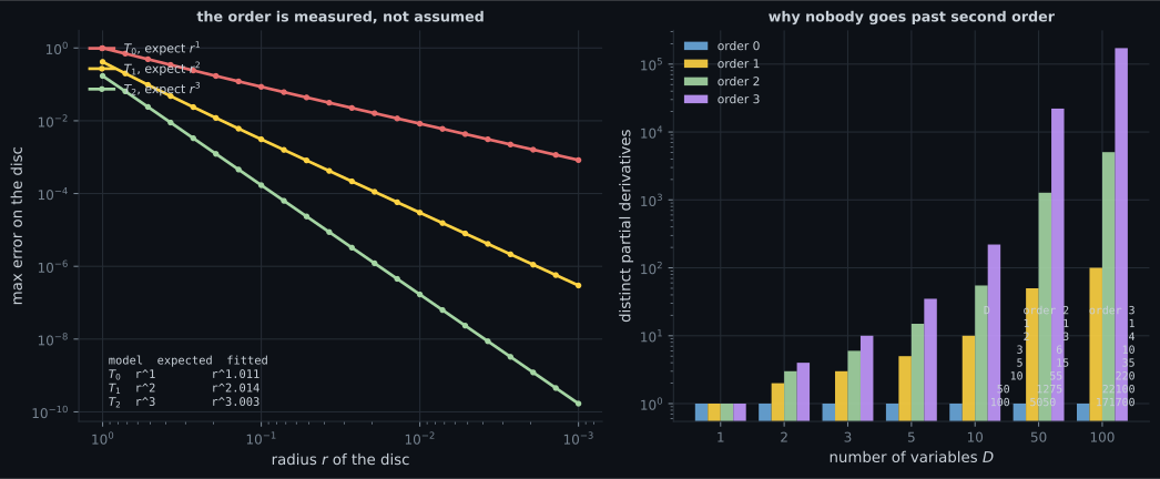
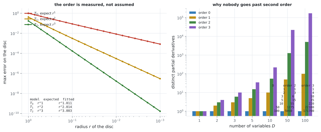
Nothing has gone wrong. Definition 5.8 promises an error that vanishes like $r^{n+1}$ as $r \to 0$, and the fitted slopes confirm it exactly: $1.067$, $2.005$, $3.019$ against the predicted $1$, $2$, $3$. A statement about a limit is not a statement about the window you happen to be plotting.

On real data

figure The value, the tangent plane, and the quadratic — measured on a disc matplotlib

One surface expanded at (0.7, 0.5), with each model's maximum and mean error over the unit disc printed underneath. T1 is Equation 5.148: its contours are perfectly straight and evenly spaced, which is what a plane looks like from above. T2's contours curve, and the error drops by more than an order of magnitude — but only inside the disc.

figure The order is measured, and the term count is the reason you stop matplotlib

Left: the order-k error should scale like r to the k plus one, and the fitted slopes come out at the integers rather than being asserted. Right: the cost that Equation 5.151 hides. Even after Equation 5.146's symmetry the distinct entries at order k number C(D+k-1, k) — at D = 1000000 that is 5.0e+11 at second order and 1.7e+17 at third.

figure A second-order expansion of a log-density is a Gaussian matplotlib

Expand log p to second order at the mode and exponentiate: the mean is the mode and the variance is minus one over the curvature. Measured here: mode 1.562500, curvature -1.024000, variance 0.976563, total variation distance 0.165397. And the honest failure — 5.69 percent of the Gaussian's mass sits at x below zero, where p is not defined at all. The right panel shows why: on a log scale a Gaussian is a parabola, and this log-density is not one.

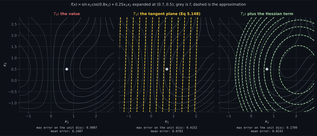
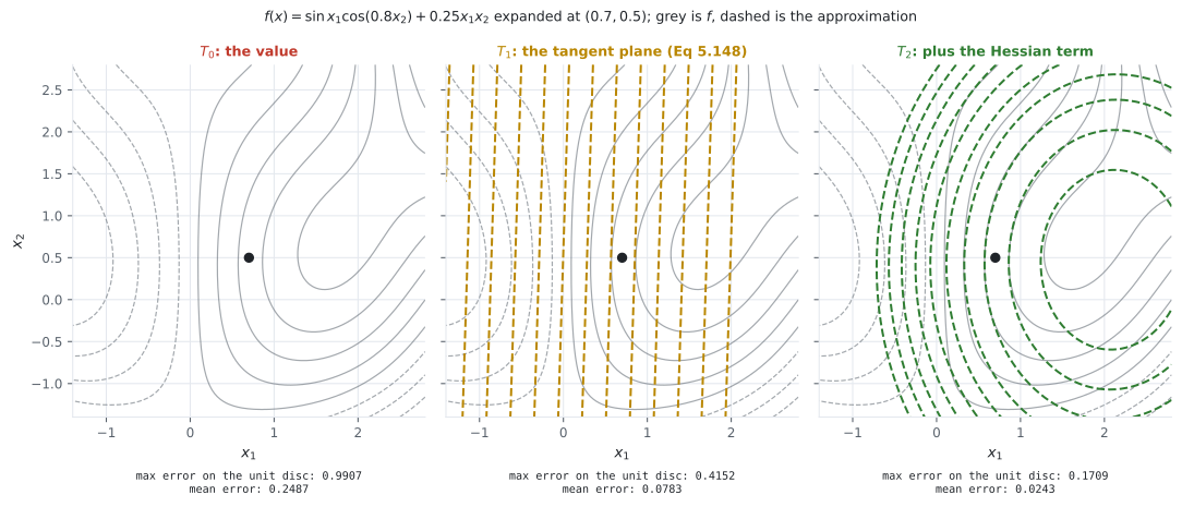
Reading the plot

From the first figure. Look at the shape of the dashed contours, not just the error numbers. $T_1$’s contours are straight and evenly spaced — that is the signature of a plane, and it tells you immediately what Equation 5.148 can and cannot represent. It cannot bend. $T_2$’s contours curve, and they curve differently along the two eigenvector directions of the Hessian, which is §5.7’s curvature showing up as geometry.

From the convergence figure. The point of fitting the slope rather than asserting it: a claim like “second-order error is $O(r^3)$” is checkable, and checking it is what distinguishes a measurement from a recital. The right-hand panel is the practical half. The bars grow combinatorially, and Equation 5.146’s symmetry — which sounds like a big saving, and is a factor of about 2 at $k=2$ — does nothing at all to the exponent.

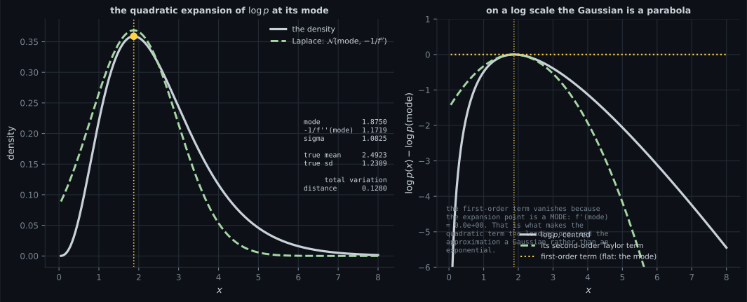
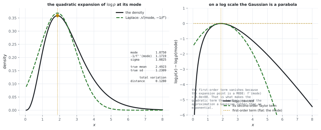
From the Laplace figure. The left panel looks like a decent fit and the right panel shows that it is not. On a log axis a Gaussian must be an exact parabola; the true log-density is visibly not one, and the mismatch is systematic in the tails rather than random. A second-order expansion matches exactly two things — the location of the mode and the curvature there — and is silent about skew, tails, and support.

From the book

Mathematics for Machine Learning, §5.8. Equation 5.148 is the linear approximation, with Figure 5.12 showing the univariate case expanded at $x_0 = -2$ and the observation that it worsens away from $x_0$. Definition 5.7 (Equations 5.149–5.151) defines the multivariate Taylor series with $\boldsymbol{\delta} := \mathbf{x} - \mathbf{x}_0$; Definition 5.8 (Equation 5.152) the Taylor polynomial of degree $n$. The book flags $\boldsymbol{\delta}^k$ as “slightly sloppy notation” and defines it as a $k$-fold outer product (Equations 5.153, 5.154, drawn in Figure 5.13), giving the general contraction in Equation 5.155 and the first four terms explicitly in Equations 5.156 to 5.160 — with the np.einsum calls in the margin. Example 5.15 (Equations 5.161–5.180) expands $x^2 + 2xy + y^3$ at $(1,2)$ and observes that the result is exact, since the original function was a third-order polynomial.

Pitfalls

Higher order is not uniformly better

It is better as the radius goes to zero, which is a different claim. Measured on a non-polynomial expanded at $(0.4, -0.3)$: at $r = 0.05$ the error ratios are $T_1/T_0 = 0.138$ and $T_2/T_1 = 0.010$; at $r = 3.2$ they are $1.573$ and $3.537$, so $T_2$‘s error of $7.77$ is five times $T_0$‘s $1.40$. If you fit a second-order model and evaluate it far from the expansion point, adding the Hessian term can actively hurt.

The cross term keeps a factor of 2

Equation 5.159’s double sum runs over all ordered pairs, so $H[1,2]$ is counted at $(1,2)$ and again at $(2,1)$. Expanding $\tfrac{1}{2}\boldsymbol{\delta}^\top H\boldsymbol{\delta}$ by hand for Example 5.15 gives $(x-1)^2 + 2(x-1)(y-2) + 6(y-2)^2$ — note the $2$ on the middle term and no $\tfrac{1}{2}$ anywhere. Writing $\tfrac{1}{2}\left(H_{11}\delta_1^2 + H_{12}\delta_1\delta_2 + H_{22}\delta_2^2\right)$ is wrong by a factor of two on exactly one term, which is the hardest kind of error to spot.

Do not build delta delta-transpose

Equation 5.158’s trace form is the right way to state the term and the wrong way to compute it. $\boldsymbol{\delta}\boldsymbol{\delta}^\top$ is a $D \times D$ matrix of rank one — at $D = 10^6$ that is $10^{12}$ entries to allocate in order to extract a single scalar. Compute $\boldsymbol{\delta}^\top(H\boldsymbol{\delta})$ instead: two matrix-vector products and no intermediate bigger than $D$. Both forms are verified to agree exactly below.

A Taylor polynomial is not a Taylor series

Equation 5.152 is a finite sum and always exists for a smooth $f$. Equation 5.151 is an infinite sum that need not converge to $f$ at any given $\mathbf{x}$, even when $f$ is infinitely differentiable. The sigmoid lab above shows the practical version: every added degree improves the fit near the expansion point and worsens the tails, and no degree fixes the tails. Never assume that a series which is valid near $\mathbf{x}_0$ describes $f$ on the domain you care about.

The Laplace approximation does not know the support

Expanding $\log p$ to second order at its mode gives a Gaussian with mean at the mode and variance $-1/H$. That Gaussian lives on all of $\mathbb{R}$. Measured on a density supported on $x > 0$: 5.69 percent of the approximation’s mass sits at $x < 0$, where the true density is not merely small but undefined. If the quantity is a variance, a count, or a probability, the approximation will happily assign it impossible values. And the expansion must be taken at a maximum — at any point where the curvature of $\log p$ is not negative, $\exp$ of the quadratic model is not integrable and there is no Gaussian at all.

Compare

	$T_1$, Equation 5.148	$T_2$	$T_3$ and beyond
Needs	$f$, $\nabla f$	plus $H$	plus an order-3 tensor
Entries at $D = 10^6$	$10^6$	$5.0 \times 10^{11}$ distinct	$1.7 \times 10^{17}$ distinct
Error as $r \to 0$	$O(r^2)$, measured $2.005$	$O(r^3)$, measured $3.019$	$O(r^4)$
Geometry	a plane; contours straight and evenly spaced	a bowl or saddle	no simple picture
Used for	Gauss–Newton, delta method, linearized filters	Newton’s method, Laplace approximation, trust regions	essentially never

Application	What it is, in §5.8’s terms
Tangent plane / linearization	$T_1$, Equation 5.148, verbatim
Newton’s method	minimise $T_2$ instead of $f$, then re-expand
Laplace approximation	$T_2$ of $\log p$ at the mode, exponentiated
Gauss–Newton	$T_1$ of the residual, then solve the resulting least squares
Delta method (statistics)	$T_1$ of a transform, to propagate a variance
Trust-region methods	$T_2$, plus an explicit bound on $\|\boldsymbol{\delta}\|$ — a direct admission that the model is only local

pch.quizTag Check your understanding

1. In Equation 5.151, what is delta-to-the-k when delta is a vector and k = 2?

   A Each component squared B The 2-fold outer product delta delta-transpose, a D by D matrix whose (i,j) entry is delta-i times delta-j — Equation 5.153 C The squared norm of delta D The matrix product of delta with itself
   pch.quizShowAnswer

   B — The 2-fold outer product delta delta-transpose, a D by D matrix whose (i,j) entry is delta-i times delta-j — Equation 5.153 — The book calls delta-to-the-k 'slightly sloppy notation' for exactly this reason. Both the derivative and the displacement become order-k tensors, and the term is a full contraction of the two — Equation 5.155.

2. Equation 5.158 writes the second-order term two ways: trace(H delta delta-transpose) and delta-transpose H delta. How do they compare?

   A The trace form is more accurate B They are the same number, but the trace form builds a D by D rank-one intermediate — so state it that way and compute the quadratic form instead C They differ by a factor of two D The trace form only works for symmetric H
   pch.quizShowAnswer

   B — They are the same number, but the trace form builds a D by D rank-one intermediate — so state it that way and compute the quadratic form instead — Verified to 0.0e+00 at four displacements. The trace form is the one that generalises to arbitrary k; the quadratic form never allocates anything bigger than D, which at a million parameters is the difference between a vector and 4 TB.

3. Example 5.15's T3 reproduces f exactly. Where is that true?

   A Only near the expansion point (1, 2) B Everywhere. f is a cubic and a degree-3 Taylor polynomial has room for every term a cubic has — checked over a grid spanning [-4, 6], max error 0.0000, and at (6, -4) both give exactly -76 C Only for the first three terms D Only where the third derivative is nonzero
   pch.quizShowAnswer

   B — Everywhere. f is a cubic and a degree-3 Taylor polynomial has room for every term a cubic has — checked over a grid spanning [-4, 6], max error 0.0000, and at (6, -4) both give exactly -76 — This is the one situation where 'Taylor expansion' and 'algebraic rearrangement' coincide. Note how little T2 buys over T1 on that same wide grid — 216 against 225 — which is the locality of a truncated series showing itself.

4. On a non-polynomial expanded at a point, the error ratio T2/T1 was measured at 0.010 for radius 0.05 and 3.537 for radius 3.2. What does that mean?

   A The Hessian was computed incorrectly B Nothing is wrong: Definition 5.8 promises an error vanishing like r-to-the-(n+1) as r goes to zero, and the fitted slopes confirm 1.067, 2.005 and 3.019 — but on a fixed large window the higher-order model can be, and here is, much worse C The function is not smooth D The expansion point was badly chosen
   pch.quizShowAnswer

   B — Nothing is wrong: Definition 5.8 promises an error vanishing like r-to-the-(n+1) as r goes to zero, and the fitted slopes confirm 1.067, 2.005 and 3.019 — but on a fixed large window the higher-order model can be, and here is, much worse — At r = 3.2 T2's error of 7.77 is five times T0's 1.40. 'Higher order is better' is a statement about a limit, and it is routinely misread as a statement about the plot in front of you.

5. Why does practice essentially never go past second order?

   A Third derivatives do not exist for most functions B The term count. The order-k tensor has D-to-the-k entries and C(D+k-1, k) distinct ones after Equation 5.146's symmetry — at D = 1000000 that is 5.0e+11 at k = 2 (4 TB in float32) and 1.7e+17 at k = 3 C The factorials in Equation 5.151 make higher terms negligible D Automatic differentiation cannot compute them
   pch.quizShowAnswer

   B — The term count. The order-k tensor has D-to-the-k entries and C(D+k-1, k) distinct ones after Equation 5.146's symmetry — at D = 1000000 that is 5.0e+11 at k = 2 (4 TB in float32) and 1.7e+17 at k = 3 — Symmetry cuts the k = 2 count roughly in half and does nothing to the exponent. The factorials do not save you either — they are constants against a combinatorial growth in the number of terms.

🧪 Try It Yourself

Exercise 1 – Linearize a function

pch.exerciseTag pch.exerciseTitle

Exercise 2 – The two forms of Equation 5.158

pch.exerciseTag pch.exerciseTitle

Exercise 3 – Contract a third-order tensor

pch.exerciseTag pch.exerciseTitle

Exercise 4 – Watch T2 stop helping

pch.exerciseTag pch.exerciseTitle

Exercise 5 – A Laplace approximation

pch.exerciseTag pch.exerciseTitle

Recall card

• Equation 5.148 is T1. f(x) is approximately f(x0) plus grad f(x0) times (x - x0), and the shapes work with no transposes precisely because §5.2 made the gradient a row.
• Definition 5.7’s delta-to-the-k is a k-fold OUTER product, not a power. Equations 5.153 and 5.154: delta-squared is delta delta-transpose with entries delta-i delta-j, delta-cubed is a D by D by D cube.
• Order-k derivatives are order-k tensors, and the term is a full contraction, Equation 5.155 — one index of the tensor paired with one copy of delta.
• The book’s margin gives the code. One index letter per order, one d per copy: einsum(“i,i”), einsum(“ij,i,j”), einsum(“ijk,i,j,k”).
• Equation 5.158’s two forms agree exactly — trace(H delta delta-transpose) equals delta-transpose H delta, verified to 0.0e+00 — but only the second should be computed. The first allocates a D by D rank-one matrix to produce one scalar.
• The cross term keeps a factor of 2, because Equation 5.159’s double sum counts (i,j) and (j,i) separately. Example 5.15’s quadratic term is (x-1)^2 + 2(x-1)(y-2) + 6(y-2)^2.
• Example 5.15 reproduces exactly. f(1,2) = 13, grad = [6 14], H = [[2,2],[2,12]], and one nonzero third derivative d3f/dy3 = 6 out of eight tensor slots.
• T3 IS f for a cubic, everywhere. Checked over a grid spanning [-4, 6]: max error 0.0000, and at (6,-4) — a displacement of 7.81 — both give exactly -76. Note T2 beat T1 by only 216 to 225 on that same grid: truncation is a LOCAL promise.
• Higher order is better only as r goes to zero. Measured error ratios T2/T1 of 0.010 at r = 0.05 and 3.537 at r = 3.2, where T2’s error of 7.77 is five times T0’s 1.40.
• The order itself is measurable. Fitted slopes 1.067, 2.005 and 3.019 against the predicted 1, 2 and 3 for T0, T1 and T2.
• The term count is why practice stops at n = 2. D-to-the-k entries, C(D+k-1, k) distinct after Equation 5.146’s symmetry — 5.0e+11 at D = 1e6 and k = 2, which is 4 TB in float32, and 1.7e+17 at k = 3. Symmetry halves the constant and does nothing to the exponent.
• The Laplace approximation is T2 of log p at the mode, exponentiated. A parabola becomes a Gaussian: mean at the mode, variance -1 over the curvature. Measured: mode 1.562500, curvature -1.024000, variance 0.976563, total variation 0.165397.
• And it does not know the support. 5.69 percent of that Gaussian’s mass sits at x below zero, where the true density is undefined — and away from a maximum, where the curvature is not negative, there is no Gaussian at all.
• A Taylor polynomial always exists; a Taylor series need not converge to f. Equation 5.152 is finite and safe. Equation 5.151 is a limit, and every added degree can improve the centre while worsening the tails.

Next: Vector Calculus Overview — the whole chapter on one page, and where each piece is used in the chapters that follow.