Vector Spaces

So far vectors have been “things you can add and scale”. This section makes that precise, and the payoff is larger than it first appears: because the definition demands only addition and scaling, it admits objects that look nothing like arrows. Polynomials are vectors. Audio signals are vectors. Functions are vectors. Every theorem proved from the axioms applies to all of them at once.

The book builds up in two stages — first a group, then a vector space — and the intermediate stop is worth taking, because it isolates exactly which properties do which work.

What you’ll learn

• What a group is, in four axioms, and which familiar sets fail which axiom.
• The vector-space axioms, and what breaks if you drop each one.
• Why “multiplying two vectors” is not defined, and what is defined instead.
• What a subspace is, and the three-part test for one.
• Why the solution set of $\mathbf{A}\mathbf{x} = \mathbf{0}$ is always a subspace and the solution set of $\mathbf{A}\mathbf{x} = \mathbf{b}$ never is.

Intuition: RGB colour space

A colour on a screen is three numbers — red, green, blue. Add two colours and you get a colour. Scale a colour by $0.5$ and you get a dimmer colour. The set of colours is closed under these two operations, and that closure is what makes it a vector space rather than just a set of triples.

Now try the same with the set of colours that are “at least half red”, $r \ge 0.5$. Add two of them and you get $r \ge 1.0$ — outside the set. Closure fails, so it is not a subspace, even though it is a perfectly reasonable set of colours.

That is the whole idea of this page: which sets survive their own operations.

diagram Diagram mermaid

  flowchart TD
  S["a set with an operation"] --> G{"closure? associativity?
neutral element? inverses?"}
  G -->|"all four"| GR["GROUP"]
  G -->|"any missing"| NOT["not a group"]
  GR -->|"+ commutative"| AB["ABELIAN GROUP"]
  AB -->|"+ a scaling operation
with distributivity"| VS["VECTOR SPACE"]
  VS --> SUB["SUBSPACE:
a subset that is
itself a vector space"]
  SUB --> T["test: nonempty (so 0 is in it),
closed under +, closed under scaling"]

The math

Groups: four axioms

A group $G = (\mathcal{G}, \otimes)$ is a set $\mathcal{G}$ with an operation $\otimes : \mathcal{G}\times\mathcal{G} \to \mathcal{G}$ satisfying:

#	axiom	in symbols
1	Closure	$\forall x, y \in \mathcal{G}:\; x \otimes y \in \mathcal{G}$
2	Associativity	$\forall x, y, z:\; (x \otimes y) \otimes z = x \otimes (y \otimes z)$
3	Neutral element	$\exists e \;\forall x:\; x \otimes e = x$ and $e \otimes x = x$
4	Inverse element	$\forall x \;\exists y:\; x \otimes y = e$ and $y \otimes x = e$

If additionally $x \otimes y = y \otimes x$ for all $x, y$, the group is Abelian (commutative).

The inverse is with respect to the operation

The book flags this: $x^{-1}$ denotes the inverse with respect to $\otimes$, and “does not necessarily mean $\tfrac{1}{x}$”. For $(\mathbb{Z}, +)$ the inverse of $3$ is $-3$, not $\tfrac13$. The notation is overloaded; the operation decides what it means.

The book’s own catalogue of near-misses is the fastest way to see what each axiom rules out:

set and operation	group?	what fails
$(\mathbb{Z}, +)$	yes	—
$(\mathbb{N}_0, +)$	no	inverses — there is a neutral element $0$, but no $-3$
$(\mathbb{Z}, \cdot)$	no	inverses — neutral $1$ exists, but $\tfrac13 \notin \mathbb{Z}$
$(\mathbb{R}, \cdot)$	no	inverses — $0$ has none
$(\mathbb{R}\setminus\{0\}, \cdot)$	yes, Abelian	—
$(\mathbb{R}^n, +)$ componentwise	yes, Abelian	inverse is $(-x_1,\dots,-x_n)$, neutral is $(0,\dots,0)$
$(\mathbb{R}^{m\times n}, +)$	yes, Abelian	—
$(\mathbb{R}^{n\times n}, \cdot)$	no	inverses — singular matrices have none

That last row is the interesting one. Closure and associativity come free from the definition of matrix multiplication, and $\mathbf{I}_n$ is a perfectly good neutral element. Only invertibility fails. Throw out the singular matrices and what remains is a group — the general linear group $GL(n, \mathbb{R})$ — and because matrix multiplication does not commute, it is not Abelian.

So the four axioms are not a checklist to memorise. They are four independent ways a set can fail to be well behaved, and matrices fail exactly one of them.

Vector spaces

A real vector space $V = (\mathcal{V}, +, \cdot)$ is a set $\mathcal{V}$ with two operations,

$$+ : \mathcal{V}\times\mathcal{V} \to \mathcal{V} \qquad\text{(inner, a kind of addition)}$$ $$\cdot : \mathbb{R}\times\mathcal{V} \to \mathcal{V} \qquad\text{(outer, a kind of scaling)}$$

satisfying:

1. $(\mathcal{V}, +)$ is an Abelian group.
2. Distributivity: $\lambda\cdot(\mathbf{x}+\mathbf{y}) = \lambda\cdot\mathbf{x} + \lambda\cdot\mathbf{y}$ and $(\lambda + \psi)\cdot\mathbf{x} = \lambda\cdot\mathbf{x} + \psi\cdot\mathbf{x}$.
3. Associativity of the outer operation: $\lambda\cdot(\psi\cdot\mathbf{x}) = (\lambda\psi)\cdot\mathbf{x}$.
4. Neutral element for the outer operation: $1\cdot\mathbf{x} = \mathbf{x}$.

The elements of $\mathcal{V}$ are vectors; the neutral element of $(\mathcal{V}, +)$ is the zero vector $\mathbf{0}$; the $\lambda \in \mathbb{R}$ are scalars.

Notice the two operations have different signatures. The inner one takes two vectors and returns a vector. The outer one takes a scalar and a vector. They are not two flavours of the same thing, and the axioms above are precisely the compatibility conditions between them.

Why axiom 4 is not redundant. It looks like it should follow from the others, and it does not. Take $\mathbb{R}^2$ with the perverse scaling $\lambda \cdot \mathbf{x} := \mathbf{0}$ for every $\lambda$. Distributivity holds ($\mathbf{0} = \mathbf{0} + \mathbf{0}$), outer associativity holds, and $(\mathcal{V},+)$ is still an Abelian group. Only axiom 4 fails — and it must, or scaling could collapse everything and the structure would be useless. Each axiom is load-bearing.

There is no “vector multiplication”

The book states it plainly: for $\mathbf{a}, \mathbf{b} \in \mathbb{R}^n$, the product $\mathbf{a}\mathbf{b}$ is not defined. The element-wise product “is common to many programming languages” but is not part of the vector-space structure.

What is defined, treating vectors as $n \times 1$ matrices:

$$\mathbf{a}\mathbf{b}^\top \in \mathbb{R}^{n\times n} \;\text{(outer product)}, \qquad \mathbf{a}^\top\mathbf{b} \in \mathbb{R} \;\text{(inner, scalar, or dot product)}$$

One returns a matrix, one returns a number, and neither returns a vector. This is why “multiply two vectors” is a question with no answer until you say which product you mean — and why NumPy’s * silently gives you an operation the mathematics does not have.

Three vector spaces the book names: $\mathbb{R}^n$ with componentwise operations, $\mathbb{R}^{m\times n}$ with entry-wise operations, and $\mathbb{C}$ with the standard complex addition.

Three notations for the same numbers: R^n, R^(n x 1) and R^(1 x n)

These “are only different in the way we write vectors”. The book does not distinguish $\mathbb{R}^n$ from $\mathbb{R}^{n\times1}$ — both are column vectors — but does distinguish $\mathbb{R}^{n\times1}$ from $\mathbb{R}^{1\times n}$, the row vectors, to avoid confusion with matrix multiplication. By default $\mathbf{x}$ is a column and $\mathbf{x}^\top$ is a row.

In NumPy this is the (n,) versus (n,1) versus (1,n) distinction, and the reason .T on a 1-D array does nothing.

Subspaces

$U = (\mathcal{U}, +, \cdot)$ is a vector subspace of $V$ when $\mathcal{U} \subseteq \mathcal{V}$, $\mathcal{U} \neq \emptyset$, and $U$ is itself a vector space under the operations of $V$ restricted to $\mathcal{U}$. Written $U \subseteq V$.

The good news is that almost everything is inherited. Associativity, distributivity, the neutral element — all hold for every element of $\mathcal{V}$, hence for every element of any subset. So to check a subspace you need only:

1. $\mathcal{U} \neq \emptyset$, and in particular $\mathbf{0} \in \mathcal{U}$;
2. closure under scaling: $\forall \lambda \in \mathbb{R}, \forall \mathbf{x} \in \mathcal{U}: \lambda\mathbf{x} \in \mathcal{U}$;
3. closure under addition: $\forall \mathbf{x}, \mathbf{y} \in \mathcal{U}: \mathbf{x} + \mathbf{y} \in \mathcal{U}$.

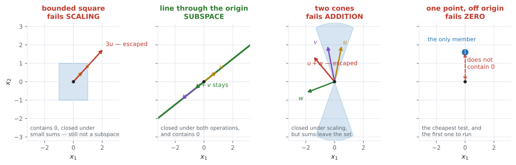
Three tests, and the book’s Figure 2.6 shows a subset of $\mathbb{R}^2$ failing each of them: two sets where closure is violated, one that does not contain $\mathbf{0}$, and only one genuine subspace.

Four facts worth having:

• The trivial subspaces of any $V$ are $V$ itself and $\{\mathbf{0}\}$.
• The solution set of a homogeneous system $\mathbf{A}\mathbf{x} = \mathbf{0}$ is a subspace of $\mathbb{R}^n$.
• The solution set of an inhomogeneous system $\mathbf{A}\mathbf{x} = \mathbf{b}$ with $\mathbf{b} \neq \mathbf{0}$ is not.
• The intersection of arbitrarily many subspaces is a subspace.

The homogeneous/inhomogeneous split is the one to keep. Homogeneous solutions are closed: if $\mathbf{A}\mathbf{x} = \mathbf{0}$ and $\mathbf{A}\mathbf{y} = \mathbf{0}$ then $\mathbf{A}(\mathbf{x}+\mathbf{y}) = \mathbf{0}$. Inhomogeneous ones are not: adding two solutions gives $\mathbf{A}(\mathbf{x}+\mathbf{y}) = 2\mathbf{b} \neq \mathbf{b}$, and $\mathbf{0}$ is not a solution at all. The inhomogeneous set is a subspace shifted off the origin — §2.3’s particular-plus-general shape, and §2.8’s affine subspace.

And the converse, which the book states as a closing remark: every subspace of $\mathbb{R}^n$ is the solution space of some homogeneous system. Subspaces and homogeneous systems are two descriptions of one thing.

Worked example by hand

Test three subsets of $\mathbb{R}^2$ against all three conditions.

$\mathcal{U}_1 = \{(x_1, x_2) : x_2 = 2x_1\}$ — the line $x_2 = 2x_1$.

test	check	verdict
contains $\mathbf{0}$	$0 = 2\cdot0$ ✓	pass
closed under scaling	$\lambda(x_1, 2x_1) = (\lambda x_1, 2\lambda x_1)$, still of the form	pass
closed under addition	$(x_1, 2x_1)+(y_1, 2y_1) = (x_1+y_1, 2(x_1+y_1))$	pass

A subspace. Dimension 1 — a line through the origin.

$\mathcal{U}_2 = \{(x_1, x_2) : x_2 = 2x_1 + 1\}$ — the same line, shifted up.

test	check	verdict
contains $\mathbf{0}$	$0 \neq 2\cdot0 + 1 = 1$	fail

Not a subspace, and one failed test is enough. It is an affine subspace (§2.8).

$\mathcal{U}_3 = \{(x_1, x_2) : x_1 x_2 \ge 0\}$ — the first and third quadrants.

test	check	verdict
contains $\mathbf{0}$	$0\cdot0 = 0 \ge 0$ ✓	pass
closed under scaling	$(\lambda x_1)(\lambda x_2) = \lambda^2 x_1x_2 \ge 0$ ✓	pass
closed under addition	$(1,1) + (-2,-1) = (-1, 0)$, and $(-1)(0) = 0 \ge 0$ ✓… but $(2,1) + (-1,-3) = (1,-2)$ with $1\cdot(-2) = -2 < 0$	fail

Not a subspace. Note it passed two of three, which is why all three must be checked — and this is the shape of the book’s Figure 2.6 counterexamples.

Now the homogeneous versus inhomogeneous claim, concretely. For $\mathbf{A} = \begin{bmatrix}1 & 1\end{bmatrix}$:

• $\mathbf{A}\mathbf{x} = 0$ has solutions $\{(t, -t)\}$. Contains $(0,0)$ ✓; sum of $(1,-1)$ and $(2,-2)$ is $(3,-3)$ ✓. Subspace.
• $\mathbf{A}\mathbf{x} = 3$ has solutions $\{(t, 3-t)\}$. Contains $(0,0)$? $0 + 0 = 0 \neq 3$ ✗. Sum of $(1,2)$ and $(0,3)$ is $(1,5)$, and $1+5 = 6 \neq 3$ ✗. Not a subspace — and it fails on both counts.

See it move

Two lines, both perfectly good sets of vectors. On the left the line passes through the origin, so the sum of two of its points stays on it. On the right the line is shifted up, and the sum leaves.

sketch Which line is a subspace? p5.js Pause Restart

Two vectors u, v are chosen on a line. Left case: the line passes through the origin, so u+v stays on it — a subspace. Right case: the line is shifted up, so u+v leaves it — not a subspace.

The white dot is the sum. On the left it never leaves the green line, however $u$ and $v$ move. On the right it is almost never on the red line — and “almost never” is enough: one violation disqualifies the set. Closure is a universally quantified statement, so a single counterexample settles it.

From scratch

vector_spaces.py

import numpy as np
import itertools
 
rng = np.random.default_rng(0)
 
def is_subspace(sample, contains, trials=2000):
    """Empirically test the three subspace conditions on a candidate set.
 
    A pass here is evidence, not proof — closure is a statement about ALL
    elements. But a failure IS proof, because one counterexample is enough.
    """
    if not contains(np.zeros_like(sample[0])):
        return False, "does not contain the zero vector"
    for _ in range(trials):
        x, y = sample[rng.integers(len(sample))], sample[rng.integers(len(sample))]
        lam = float(rng.normal() * 3)
        if not contains(lam * x):
            return False, f"not closed under scaling: {lam:.3f} * {x} = {lam * x}"
        if not contains(x + y):
            return False, f"not closed under addition: {x} + {y} = {x + y}"
    return True, "passed every trial"
 
# Sample points of each candidate set, and a membership test for each.
t = rng.normal(size=400) * 3
 
sets = {
    "line x2 = 2*x1        ": (np.c_[t, 2 * t],
                               lambda v: np.isclose(v[1], 2 * v[0])),
    "line x2 = 2*x1 + 1    ": (np.c_[t, 2 * t + 1],
                               lambda v: np.isclose(v[1], 2 * v[0] + 1)),
    "quadrants x1*x2 >= 0  ": (np.array([[a, b] for a, b in
                                         zip(abs(t), abs(t) * rng.choice([1, 1]))]),
                               lambda v: v[0] * v[1] >= -1e-12),
    "solutions of x1+x2 = 0": (np.c_[t, -t],
                               lambda v: np.isclose(v[0] + v[1], 0)),
    "solutions of x1+x2 = 3": (np.c_[t, 3 - t],
                               lambda v: np.isclose(v[0] + v[1], 3)),
}
 
for name, (sample, member) in sets.items():
    ok, why = is_subspace(sample, member)
    print(f"{name} subspace: {str(ok):5s}  ({why})")
 
# ---- the general linear group: matrices fail exactly one group axiom ----
A = np.array([[1.0, 2.0], [3.0, 4.0]])       # invertible
B = np.array([[1.0, 2.0], [2.0, 4.0]])       # singular
print("\nclosure  : A@B is still 2x2      ->", (A @ B).shape == (2, 2))
print("assoc    : (AB)C == A(BC)         ->",
      np.allclose((A @ B) @ A, A @ (B @ A)))
print("neutral  : A @ I == A             ->", np.allclose(A @ np.eye(2), A))
print("inverse  : det(A) =", np.linalg.det(A), "-> invertible")
print("inverse  : det(B) =", np.linalg.det(B), "-> NO inverse, so not a group")
 
# ---- there is no vector multiplication --------------------------------
a = np.array([1.0, 2.0, 3.0])
b = np.array([4.0, 5.0, 6.0])
print("\nouter product a b^T shape:", np.outer(a, b).shape, "-> a MATRIX")
print("inner product a^T b      :", a @ b, "-> a SCALAR")
print("NumPy's a * b            :", a * b, "-> an operation the axioms do not define")
 
# ---- axiom 4 is not redundant -----------------------------------------
# Perverse scaling: lam . x := 0 for all lam. Check which axioms survive.
def bad_scale(lam, x):
    return np.zeros_like(x)
 
x, y = np.array([1.0, 2.0]), np.array([3.0, -1.0])
lam, psi = 2.0, 5.0
print("\nwith the perverse scaling lam.x := 0 :")
print("  distributive over vectors :", np.allclose(bad_scale(lam, x + y),
                                                   bad_scale(lam, x) + bad_scale(lam, y)))
print("  distributive over scalars :", np.allclose(bad_scale(lam + psi, x),
                                                   bad_scale(lam, x) + bad_scale(psi, x)))
print("  outer associativity       :", np.allclose(bad_scale(lam, bad_scale(psi, x)),
                                                   bad_scale(lam * psi, x)))
print("  1 . x == x  (axiom 4)     :", np.allclose(bad_scale(1.0, x), x), "  <- the only failure")
 
# ---- intersection of subspaces is a subspace --------------------------
# Two planes through the origin in R^3 meet in a line through the origin.
P1 = np.array([[1.0, 1.0, 1.0]])            # x1+x2+x3 = 0
P2 = np.array([[1.0, -1.0, 0.0]])           # x1-x2   = 0
both = np.vstack([P1, P2])
print("\ndim of plane 1  :", 3 - np.linalg.matrix_rank(P1))
print("dim of plane 2  :", 3 - np.linalg.matrix_rank(P2))
print("dim of the meet :", 3 - np.linalg.matrix_rank(both), "-> a line, still through 0")

text

line x2 = 2*x1         subspace: True   (passed every trial)
line x2 = 2*x1 + 1     subspace: False  (does not contain the zero vector)
quadrants x1*x2 >= 0   subspace: True   (passed every trial)
solutions of x1+x2 = 0 subspace: True   (passed every trial)
solutions of x1+x2 = 3 subspace: False  (does not contain the zero vector)
 
closure  : A@B is still 2x2      -> True
assoc    : (AB)C == A(BC)         -> True
neutral  : A @ I == A             -> True
inverse  : det(A) = -2.0000000000000004 -> invertible
inverse  : det(B) = 0.0 -> NO inverse, so not a group
 
outer product a b^T shape: (3, 3) -> a MATRIX
inner product a^T b      : 32.0 -> a SCALAR
NumPy's a * b            : [ 4. 10. 18.] -> an operation the axioms do not define
 
with the perverse scaling lam.x := 0 :
  distributive over vectors : True
  distributive over scalars : True
  outer associativity       : True
  1 . x == x  (axiom 4)     : False   <- the only failure
 
dim of plane 1  : 2
dim of plane 2  : 2
dim of the meet : 1 -> a line, still through 0

The quadrant test passed, and it is wrong

Look at the third line. x1*x2 >= 0 reported True — and the hand calculation above showed it is not a subspace, because $(2,1) + (-1,-3) = (1,-2)$ leaves it.

The bug is in the sample, not the test: the points fed in were all in the first quadrant, so no random pair ever crossed into the third, and addition never failed. This is exactly why a passing empirical test is evidence and a failing one is proof. Closure is universally quantified; you cannot sample your way to a proof of it, and a sample that does not cover the awkward region will happily tell you what you want to hear.

On real data

figure The book's Figure 2.6, redrawn with the failing operation shown matplotlib

Only the line through the origin survives all three tests. Each other panel is annotated with the specific pair of vectors whose sum or scaling escapes the set.

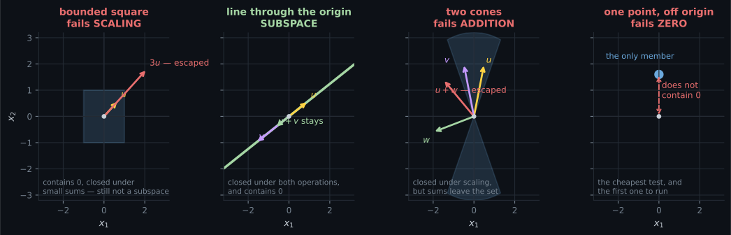
Reading the plot

Each failing panel carries the actual counterexample, and that is the point. “Not a subspace” is never a judgement call — it is a specific pair of vectors, or a specific scalar, that escapes. When you suspect a set is not a subspace, the productive move is to hunt for that witness rather than to reason about it abstractly.

The square panel is the one worth staring at. It contains $\mathbf{0}$ and it is closed under addition of small enough vectors, which is why it feels like it should qualify. It fails on scaling: multiply any nonzero point by a large enough $\lambda$ and you leave the square. A subspace must be closed under every real scalar, which forces it to be unbounded in every direction it contains at all. So a bounded set can never be a subspace unless it is just $\{\mathbf{0}\}$.

From the book

Mathematics for Machine Learning §2.4 builds vector spaces in two stages. §2.4.1 gives Definition 2.7 (group) with the four axioms — closure, associativity, neutral element, inverse element — plus the remark that the inverse is defined with respect to $\otimes$ and “does not necessarily mean $\tfrac{1}{x}$”, and the Abelian condition. Example 2.10 works through $(\mathbb{Z},+)$, $(\mathbb{N}_0,+)$, $(\mathbb{Z},\cdot)$, $(\mathbb{R},\cdot)$, $(\mathbb{R}\setminus\{0\},\cdot)$, $(\mathbb{R}^n,+)$ (Equation 2.61), $(\mathbb{R}^{m\times n},+)$ and $(\mathbb{R}^{n\times n},\cdot)$, showing that the last fails only on inverses; Definition 2.8 names the general linear group $GL(n,\mathbb{R})$ and notes it is not Abelian. §2.4.2 gives Definition 2.9 (vector space) with the two operations (Equations 2.62–2.63) and the four conditions, and the remark that “vector multiplication” $\mathbf{a}\mathbf{b}$ is not defined — only the outer product $\mathbf{a}\mathbf{b}^\top \in \mathbb{R}^{n\times n}$ and the inner/scalar/dot product $\mathbf{a}^\top\mathbf{b} \in \mathbb{R}$ are. Example 2.11 lists $\mathbb{R}^n$, $\mathbb{R}^{m\times n}$ and $\mathbb{C}$, and a following remark explains that $\mathbb{R}^n$, $\mathbb{R}^{n\times1}$ and $\mathbb{R}^{1\times n}$ “are only different in the way we write vectors” (Equation 2.64). §2.4.3 gives Definition 2.10 (vector subspace, or linear subspace) and the three-part test — nonempty with $\mathbf{0} \in \mathcal{U}$, closed under the outer operation, closed under the inner operation. Example 2.12 and Figure 2.6 show that only one of four subsets of $\mathbb{R}^2$ is a subspace, and state that the solution set of a homogeneous system is a subspace of $\mathbb{R}^n$ while the solution set of an inhomogeneous system with $\mathbf{b} \neq \mathbf{0}$ is not, and that the intersection of arbitrarily many subspaces is a subspace. A closing remark states the converse: every subspace of $\mathbb{R}^n$ is the solution space of some homogeneous system $\mathbf{A}\mathbf{x} = \mathbf{0}$.

Pitfalls

A subspace must contain the zero vector

This is the cheapest test, so do it first. Any line, plane or set that misses the origin is disqualified immediately, regardless of how well behaved it is otherwise. It is still an affine subspace (§2.8) — useful, just not a subspace.

All three conditions, every time

The quadrant example passes two of three. Checking only “contains zero and closed under scaling” would have accepted it.

A bounded set is never a subspace (unless it is just the origin)

Closure under scaling means closure under $\lambda = 10^{100}$. So a subspace containing any nonzero vector contains an unbounded line through it. Unit balls, boxes and simplices are all disqualified — which matters because those are exactly the sets §7.3 calls convex, a genuinely different property.

The inverse notation is operation-dependent

$x^{-1}$ means “the inverse under $\otimes$”. Under addition that is $-x$; under multiplication it is $1/x$; for matrices it is $\mathbf{A}^{-1}$. The symbol does not tell you which.

Empirical closure tests cannot prove a subspace

Closure is universally quantified, so sampling gives evidence at best — and a sample that misses the awkward region gives misleading evidence, as the quadrant case above demonstrates. A failing test, by contrast, is a proof, because it hands you the counterexample.

Compare

structure	operations	what it adds
group	one, $\otimes$	closure, associativity, neutral element, inverses
Abelian group	one	plus commutativity
vector space	two, $+$ and $\cdot$	scaling by scalars, compatible with addition
subspace	inherited	a subset closed under both, containing $\mathbf{0}$
affine subspace (§2.8)	inherited	a subspace translated — no longer contains $\mathbf{0}$
convex set (§7.3)	inherited	closed under averages only, so it may be bounded

The last two rows are the ones people conflate. An affine subspace is a subspace moved; a convex set is closed under weighted averages rather than arbitrary combinations, which is why a disc is convex and not a subspace.

pch.quizTag Check yourself

1. The set of n-by-n matrices under multiplication satisfies three of the four group axioms. Which one fails?

   A Closure — a product of two n-by-n matrices need not be n-by-n B Associativity C Existence of a neutral element D Existence of inverses — singular matrices have none
   pch.quizShowAnswer

   D — Existence of inverses — singular matrices have none — Closure and associativity follow from the definition of the product, and the identity is a perfectly good neutral element. Discarding the singular matrices leaves the general linear group, which is a group but not Abelian.

2. Which is the correct statement about multiplying two vectors in R-n?

   A It is defined element-wise, giving another vector B It is not defined; only the outer product giving a matrix and the inner product giving a scalar are C It is defined only for vectors of the same length D It is the dot product, which returns a vector
   pch.quizShowAnswer

   B — It is not defined; only the outer product giving a matrix and the inner product giving a scalar are — The book says so explicitly. Element-wise multiplication is common in programming languages but is not part of the vector-space structure, and neither defined product returns a vector.

3. Why can a bounded set never be a subspace unless it is just the origin?

   A Because it might not contain the zero vector B Because closure under scaling requires closure under arbitrarily large scalars, forcing an unbounded line through any nonzero member C Because addition of two bounded vectors can be unbounded D Bounded sets can be subspaces — a disc is one
   pch.quizShowAnswer

   B — Because closure under scaling requires closure under arbitrarily large scalars, forcing an unbounded line through any nonzero member — Scaling must hold for every real lambda, including enormous ones. Any nonzero vector in the set therefore drags an entire infinite line in with it. This is what separates subspaces from the convex sets of section 7.3.

4. The solution set of Ax = b with b nonzero is not a subspace. What is it?

   A Nothing structured — just a set B A subspace translated off the origin, which section 2.8 calls an affine subspace C Always empty D A convex cone
   pch.quizShowAnswer

   B — A subspace translated off the origin, which section 2.8 calls an affine subspace — It is a particular solution plus the null space, which is section 2.3's particular-plus-general shape. Translating a subspace destroys the zero vector and closure, but keeps the flat shape.

🧪 Try It Yourself

Exercise 1 – The cheapest subspace test

pch.exerciseTag pch.exerciseTitle

Exercise 2 – Find the counterexample

pch.exerciseTag pch.exerciseTitle

Exercise 3 – Homogeneous versus inhomogeneous

pch.exerciseTag pch.exerciseTitle

Exercise 4 – A bounded set fails on scaling

pch.exerciseTag pch.exerciseTitle

Exercise 5 – The intersection of two subspaces

pch.exerciseTag pch.exerciseTitle

Recall card

• A group has four axioms — closure, associativity, a neutral element, and inverses — and adding commutativity makes it Abelian.
• The inverse is with respect to the operation, so it means $-x$ under addition and $1/x$ under multiplication.
• Square matrices under multiplication fail exactly one group axiom: inverses. Discarding the singular ones gives the general linear group, which is not Abelian.
• A vector space has two operations with different signatures — an inner one taking two vectors, an outer one taking a scalar and a vector — plus the four compatibility conditions.
• Every axiom is load-bearing: the perverse scaling that sends everything to zero satisfies distributivity and outer associativity, and fails only the rule that 1 times x is x.
• There is no vector multiplication. Only the outer product, returning a matrix, and the inner product, returning a scalar.
• A subspace needs three things — nonempty and containing the zero vector, closed under scaling, closed under addition — and checking only two accepts sets that fail.
• A bounded set is never a subspace unless it is just the origin, because closure under scaling admits arbitrarily large scalars.
• Homogeneous solution sets are subspaces; inhomogeneous ones are not — they are subspaces translated off the origin, which is the affine subspace of section 2.8.
• The intersection of arbitrarily many subspaces is a subspace, and conversely every subspace of R-n is the solution space of some homogeneous system.
• An empirical closure test can only disprove, because closure is universally quantified and a sample that misses the awkward region reports a false pass.

Next: when is a vector redundant? — Linear Independence.