
Capstone 5 - A Recommender with an Honest Evaluation
The decision
Section titled “The decision”A catalogue of 600 items, 1,200 users, and a slot on the home page showing ten recommendations. The questions the team actually has to answer:
- Is a personalised recommender worth building at all, against showing the most popular items?
- Which users should it be applied to?
- How do we know the offline number is not a fantasy?
The third question is the hard one, and it is why this capstone exists. The recommender page measured that evaluating against 100 sampled negatives instead of the full catalogue inflates every hit rate by 1.90× to 2.14×. Every number below is a full-catalogue number.
Step 1 — the protocol, decided before the model
Section titled “Step 1 — the protocol, decided before the model”| Choice | Decision | Why |
|---|---|---|
| split | leave-one-out per user with ≥5 interactions | matches “predict the next thing” |
| evaluable users | 1,017 of 1,200 | 183 users have too little history |
| candidates | all 600 items, minus the ones the user already has | sampling inflates by ~2× |
| metric | hit rate at 5, 10 and 20 | 10 is the slot size; the others show sensitivity |
| second metric | catalogue coverage | a recommender that shows 20 items is not a recommender |
| baseline | most popular items | it must be beaten before anything ships |
Writing this table first is the whole trick. Every reported improvement in recommender systems is negotiable if the protocol is chosen after the results.
Step 2 — the results
Section titled “Step 2 — the results”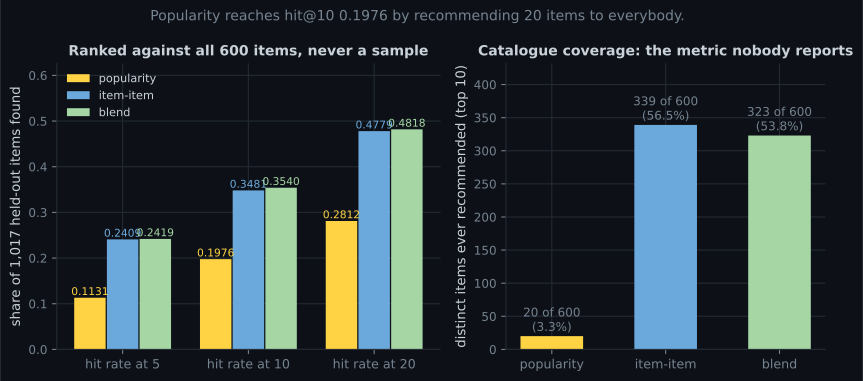
| Policy | hit@5 | hit@10 | hit@20 | Catalogue coverage (top 10) |
|---|---|---|---|---|
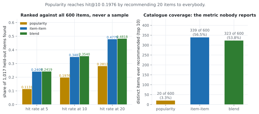
| popularity | 0.1131 | 0.1976 | 0.2812 | 20 of 600 (3.3%) |
| item-item cosine | 0.2409 | 0.3481 | 0.4779 | 339 of 600 (56.5%) |
| blend | 0.2419 | 0.3540 | 0.4818 | 323 of 600 (53.8%) |
Personalisation is worth building here. hit@10 goes from 0.1976 to 0.3481 — a 1.76× improvement, measured against the full catalogue, using six lines of numpy.
Catalogue coverage is the finding nobody asks for. Popularity’s 0.1976 comes from recommending the same 20 items to all 1,017 users. As an accuracy metric that is fine; as a product it means 96.7% of the catalogue is never seen, new items can never be discovered, and every user’s home page looks identical. Report coverage next to hit rate, always.
Step 3 — the blend, and where it comes from
Section titled “Step 3 — the blend, and where it comes from”The cold-start measurement showed that personalisation loses on users with almost no history. So the policy is two lines:
def scores_for(user):
    """Popularity for cold users, collaborative filtering for everyone else."""
    if interactions_in_training[user] < MIN_HISTORY:      # 5
        return popularity
return train[user] @ item_similarity| Interactions in training | n | popularity | item-item | blend |
|---|---|---|---|---|
| 4 | 81 | 0.2469 | 0.1728 | 0.2469 |
| 5–7 | 252 | 0.2421 | 0.3135 | 0.3135 |
| 8–10 | 199 | 0.2060 | 0.3266 | 0.3266 |
| 11–15 | 203 | 0.2118 | 0.4138 | 0.4138 |
| 16–61 | 282 | 0.1277 | 0.3972 | 0.3972 |
| all | 1,017 | 0.1976 | 0.3481 | 0.3540 |
The blend gains +0.0059 overall, and all of it comes from the 81 users where item-item scored 0.1728 and popularity scored 0.2469. That is a small aggregate number produced by a large segment-level one — +0.0741 for the users it affects — which is the shape most good production changes have.
See it move
Section titled “See it move”MIN_HISTORY is the only parameter in that policy, and it is a routing parameter rather than a model
one — so its effect can be computed exactly from the segment table. Drag it and watch each segment
switch strategy and the aggregate follow.
The weighted average reproduces the published numbers exactly, which is a useful check that the blend is arithmetic rather than magic: cutoff 0 gives 0.3481 (item-item everywhere), cutoff 5 gives 0.3540 (the blend), and cutoff 62 gives 0.1976 (popularity everywhere). Push the cutoff past 5 and the aggregate falls — 0.3363 at 8, 0.3127 at 11, 0.2724 at 16 — because you are now handing popularity to users who have enough history for personalisation to win. The optimum sits exactly where the two per-segment bars cross, and nowhere else.
Step 4 — what the online system needs
Section titled “Step 4 — what the online system needs”CONFIG = {"slate_size": 10, "min_history": 5, "model_version": "reco-3.0.1"}
def recommend(user_id, artefact, config):
"""A slate, plus the fields that make an offline/online comparison possible."""
history = artefact["history"](user_id)
cold = len(history) < config["min_history"]
scores = (artefact["popularity"] if cold
else artefact["similarity_scores"](history))
ranked = [item for item in np.argsort(-scores) if item not in history]
slate = ranked[:config["slate_size"]]
return {
"user_id": user_id,
"slate": slate,
"strategy": "popularity" if cold else "item_item",
"history_size": len(history),
"score_span": round(float(scores[slate[0]] - scores[slate[-1]]), 6),
"model_version": config["model_version"],
"catalogue_share_today": artefact["coverage_counter"].add(slate),
}Three of those fields exist because of what this phase measured. strategy makes the blend auditable
— when the cold-user share moves, the aggregate hit rate moves with it and you need to know which. **
score_span** is near zero when the model has nothing to say, which is a better abstention signal than a
threshold on the raw score. catalogue_share_today is coverage as a live metric rather than an
offline curiosity.
Step 5 — the honest limits of the offline number
Section titled “Step 5 — the honest limits of the offline number”| Problem | Why the offline number is optimistic | What to do |
|---|---|---|
| Feedback loops | Yesterday’s recommendations created today’s interactions, so the model is scored on data it shaped | Log which slate produced each interaction; hold out a random-slate slice |
| Position bias | Item 1 is clicked more than item 10 regardless of relevance | Model position explicitly, or randomise within the slate |
| Only one relevant item | Leave-one-out treats the other 599 as irrelevant, which is false | Report it as a lower bound; run an online test |
| 183 excluded users | 15% of the base has too little history to evaluate at all | Their metric is a product question: what does a new user see? |
| No timestamps | A random held-out item can predate the training interactions | Use a temporal split for a production estimate |
The last two are the ones with teeth. A leave-one-out benchmark excludes exactly the users the blend was built for, and it can leak the future by holding out an early interaction. A temporal split fixes the second; nothing fixes the first except deciding, as a product, what a brand-new user sees.
Offline evaluation ranks candidate policies; it does not predict online performance. The purpose of the protocol above is to shortlist honestly, cheaply and reproducibly. The number that matters comes from an A/B test, and the offline number’s job is to make sure the A/B test is worth running.
The loop that number lives inside, with the leak that makes it optimistic drawn explicitly:
  flowchart TD
  L[("interaction log")] --> SPLIT{{"leave-one-out per user,
full 600-item ranking"}}
  SPLIT -->|"183 users have
fewer than 5 interactions"| EXCL["excluded from evaluation.
15% of the base, and exactly
the users the blend targets."]
  SPLIT --> TRAIN["fit: popularity vector
and item-item cosine"]
  TRAIN --> POL{{"blend: popularity below
5 interactions, item-item above"}}
  POL --> OFF["offline: hit@10 0.3540,
coverage 323 of 600"]
  OFF --> GATE{"Better than the
shipped policy, on both
hit rate and coverage?"}
  GATE -->|"no"| STOP["do not run the A/B test"]
  GATE -->|"yes"| AB["online A/B test --
the only number that decides"]
  AB --> SERVE["serve slates"]
  SERVE --> CLICK["users interact with
what they were shown"]
  CLICK -.->|"the feedback loop:
today's log was shaped
by yesterday's slates"| L
  SERVE -->|"small random-slate slice"| UNBIASED["unbiased evaluation data --
the only defence against
the dotted edge"]
  UNBIASED --> L
  SERVE --> POS["log slate position
per interaction"]
  POS -->|"item 1 outclicks item 10
whatever the relevance"| DEBIAS["model position explicitly,
or randomise within the slate"]
The dotted edge is why an offline hit rate cannot be a forecast: the data it is measured on was produced by the policy it is being compared against. The random-slate slice is the cheap structural fix — a few percent of traffic showing unranked items buys you an evaluation set that no policy has contaminated, and without it every future offline comparison inherits the same bias.
- 1,017 evaluable users of 1,200; every number computed against the full 600-item catalogue.
- Popularity: hit@10 0.1976 while showing only 20 distinct items (3.3% of the catalogue).
- Item-item cosine: hit@10 0.3481 across 339 items — a 1.76× improvement, in six lines.
- The blend (popularity below five interactions) reaches 0.3540, gaining +0.0741 for the 81 cold users and +0.0059 overall.
- Catalogue coverage belongs next to hit rate in every report.
- Offline numbers shortlist policies. Feedback loops, position bias and the 183 excluded users mean the decision belongs to an online test.
-
Your recommender reaches hit rate 0.1976 at 10. What must you check before calling it a success?
Two protocol facts decide the interpretation: sampled negatives inflate hit rates by about 2x, and a policy can reach a respectable hit rate while making 96.7% of the catalogue unreachable.
pch.quizShowAnswer
B — Whether that number was measured against the full catalogue, and how many distinct items the policy ever recommends — the popularity baseline hits 0.1976 while showing only 20 of 600 items — Two protocol facts decide the interpretation: sampled negatives inflate hit rates by about 2x, and a policy can reach a respectable hit rate while making 96.7% of the catalogue unreachable.
-
The blend lifts hit@10 from 0.3481 to 0.3540. Is it worth shipping?
Segmenting by activity turns an ignorable aggregate into a clear decision. This is the usual shape of a good production change: a large effect on a small, important segment.
pch.quizShowAnswer
B — Yes: the aggregate is small because the blend only affects 81 users, and for them it is worth +0.0741 — the newest users, who are also the most likely to leave — Segmenting by activity turns an ignorable aggregate into a clear decision. This is the usual shape of a good production change: a large effect on a small, important segment.
-
Why report catalogue coverage alongside hit rate?
Coverage is a product constraint that accuracy metrics are blind to. It is also cheap: count the distinct items appearing in top-10 slates, offline and in production.
pch.quizShowAnswer
B — Because a policy can score well while showing everyone the same few items — 20 of 600 here — which makes new items undiscoverable and every home page identical — Coverage is a product constraint that accuracy metrics are blind to. It is also cheap: count the distinct items appearing in top-10 slates, offline and in production.
-
Which limitation of the offline evaluation is least fixable by a better protocol?
Full-catalogue ranking fixes sampling, randomisation-within-slate mitigates position bias, and treating leave-one-out as a lower bound handles the single-relevant-item problem. Breaking the feedback loop requires deliberately logging random slates.
pch.quizShowAnswer
B — The feedback loop: the interactions you evaluate on were themselves produced by earlier recommendations, so the model is scored on data it shaped — Full-catalogue ranking fixes sampling, randomisation-within-slate mitigates position bias, and treating leave-one-out as a lower bound handles the single-relevant-item problem. Breaking the feedback loop requires deliberately logging random slates.
-
What is the correct role of the offline hit rate?
It cannot predict online performance — feedback loops and position bias make the mapping unknown. It can rank policies honestly, which is what decides where to spend a limited number of experiment slots.
pch.quizShowAnswer
B — To shortlist candidate policies cheaply and reproducibly, so that the A/B test is worth running — It cannot predict online performance — feedback loops and position bias make the mapping unknown. It can rank policies honestly, which is what decides where to spend a limited number of experiment slots.
🧪 Try It Yourself
Section titled “🧪 Try It Yourself”Exercise 1 – Set up the protocol
Section titled “Exercise 1 – Set up the protocol”Exercise 2 – Score three policies at three cut-offs
Section titled “Exercise 2 – Score three policies at three cut-offs”Exercise 3 – Count the catalogue
Section titled “Exercise 3 – Count the catalogue”Exercise 4 – Segment by activity, and find the blend’s real effect
Section titled “Exercise 4 – Segment by activity, and find the blend’s real effect”Exercise 5 – Show what the sampled protocol would have claimed
Section titled “Exercise 5 – Show what the sampled protocol would have claimed”Phase 12 - Capstone Projects — the phase overview, and the six questions every one of these projects had to answer before a model was worth building.
pch.coffeeTagline
pch.coffeeCtapch.feedbackHeading
pch.feedbackSubheading