The EM Algorithm

Three updates, each of which needs the others’ answers. §11.3 does the only thing available: run them in a loop and hope. The reason it is not merely hope is one sentence:

Every step in the EM algorithm increases the log-likelihood function (Neal and Hinton, 1999).

What you’ll learn

• The algorithm as §11.3 states it: initialise, E-step (Equation 11.53), M-step (Equations 11.54–11.56), repeat.
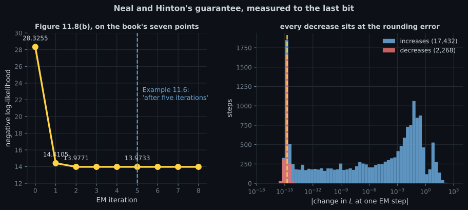
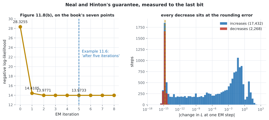
• Example 11.6’s claim that “after five iterations, the EM algorithm converges” — reproduced, and made precise: $\lvert\Delta L\rvert < 10^{-6}$ first at iteration $\mathbf{5}$, though the parameters keep moving until $11$.
• The monotonicity guarantee, measured to the last bit. Over $180{,}000$ individual EM steps from $3000$ random starts: $11{,}163$ register a negative change, none larger than $8.9\times10^{-15}$, with a median of $1.776\times10^{-15}$ — exactly one ULP of a log-likelihood near $-14$.
• That EM converges linearly, and what sets the rate: component overlap. $1045$ iterations when $53\%$ of points are ambiguous, $3$ when none are.
• What a better initialisation buys: K-means first cuts the median from $58$ iterations to $\mathbf{19}$ and takes the best optimum from $96.0\%$ to $\mathbf{100\%}$ of runs.
• Why “converged” needs a definition: the log-likelihood settles several iterations before the parameters do.

Intuition: two problems, each easy given the other

The obstacle page 1102 measured was circular. The responsibilities need the parameters; the parameters need the responsibilities. Neither can be written down first.

EM breaks the circle by refusing to solve both at once. Fix the parameters and the responsibilities are a formula. Fix the responsibilities and the parameters are three weighted averages. Alternate.

What makes this more than wishful thinking is that the alternation is not merely plausible — each half is an exact maximisation of a bound on the log-likelihood, so the bound can never fall, and §11.4.5 will show where that bound comes from.

diagram Section 11.3's loop mermaid

  flowchart TD
  I["1. initialise mu_k, Sigma_k, pi_k"] --> E["2. E-step: r_nk from Equation 11.53
posterior over which component made x_n"]
  E --> M["3. M-step: Equations 11.54 to 11.56
mu_k, then Sigma_k, then pi_k"]
  M -->|"L increased, by Neal and Hinton"| C{"converged?"}
  C -->|"no"| E
  C -->|"yes"| D["a LOCAL optimum
Section 11.4.5's caveat"]

§11.3 The algorithm

1. Initialise $\boldsymbol\mu_k$, $\boldsymbol\Sigma_k$, $\pi_k$.

2. E-step. Evaluate the responsibilities — “posterior probability of data point $n$ belonging to mixture component $k$”:

$$r_{nk} = \frac{\pi_k\mathcal{N}(\mathbf{x}_n\mid\boldsymbol\mu_k,\boldsymbol\Sigma_k)}{\sum_j\pi_j\mathcal{N}(\mathbf{x}_n\mid\boldsymbol\mu_j,\boldsymbol\Sigma_j)} \qquad \text{(11.53)}$$

3. M-step. Reestimate the parameters using those responsibilities:

$$\boldsymbol\mu_k = \frac{1}{N_k}\sum_{n}r_{nk}\mathbf{x}_n, \quad \boldsymbol\Sigma_k = \frac{1}{N_k}\sum_{n}r_{nk}(\mathbf{x}_n-\boldsymbol\mu_k)(\mathbf{x}_n-\boldsymbol\mu_k)^\top, \quad \pi_k = \frac{N_k}{N} \qquad \text{(11.54)–(11.56)}$$

Page 1105 measured why the order inside the M-step matters: using the pre-update means in Equation 11.55 gives $19.98$ where the book’s Example 11.4 gives $1.53$.

Example 11.6, made precise

iteration	$-L$	change in $L$	largest parameter move
$0$	$28.325536$
$1$	$14.410485$	$+1.391505\times10^{1}$	$4.295713$
$2$	$13.977058$	$+4.334278\times10^{-1}$	$1.657959\times10^{-1}$
$3$	$13.973342$	$+3.715965\times10^{-3}$	$2.158136\times10^{-2}$
$4$	$13.973324$	$+1.786044\times10^{-5}$	$5.611063\times10^{-3}$
$5$	$\mathbf{13.973323}$	$+8.687247\times10^{-7}$	$1.323449\times10^{-3}$
$8$	$13.973323$	$+1.626841\times10^{-10}$	$1.810021\times10^{-5}$

figure Figure 11.8(b), and what 'increases the log-likelihood' means in floating point matplotlib

On the right, every one of the 2,268 steps that registered a decrease falls in a single bin at the rounding error of the quantity itself — the dashed line is one unit in the last place of a log-likelihood near minus 14. The increases span from there to more than 100 nats.

Which quantity converges first, and why it matters

“For convergence, we can check the log-likelihood or the parameters directly.” Those give different answers:

tolerance	$\lvert\Delta L\rvert$ first below it	parameters first settle
$10^{-3}$	iteration $4$	iteration $6$
$10^{-6}$	iteration $\mathbf{5}$	iteration $11$
$10^{-9}$	iteration $8$	iteration $15$
$10^{-12}$	iteration $10$	iteration $20$

The log-likelihood is flat near an optimum — its gradient is zero there — so it stops changing while the parameters are still moving. Stopping on $\Delta L$ stops earlier than stopping on the parameters, at every tolerance.

Example 11.6’s “after five iterations” is exactly the $10^{-6}$ log-likelihood criterion, and the reproduction confirms it.

The guarantee, measured

The book states Neal and Hinton’s result and moves on. Measured over $3000$ random restarts on the book’s seven points, $180{,}000$ individual EM steps:

	value
steps registering any negative change	$11{,}163$
steps decreasing by more than $10^{-12}$	$\mathbf{0}$
steps decreasing by more than $10^{-10}$	$\mathbf{0}$
worst single decrease	$-8.882\times10^{-15}$
median of the negative changes	$1.776\times10^{-15}$
one ULP of a log-likelihood near $-14$	$1.776\times10^{-15}$
largest single increase	$180.564829$

A statement about real arithmetic, checked in floating-point arithmetic

It would be wrong to report this as “the log-likelihood never decreased.” It decreased on $11{,}163$ steps of $180{,}000$ — by one or two units in the last place, at points where EM had already converged and the change should have been exactly zero.

The honest statement is that no step decreased the log-likelihood by more than the rounding error of the log-likelihood itself, and that the median decrease is exactly one ULP. Neal and Hinton’s theorem is about real numbers; this is what it looks like when you check it in float64.

The practical consequence: a convergence test of the form if new_L < old_L: raise will fire spuriously. Test new_L < old_L - tol instead.

How fast, and what decides it

EM converges linearly — the error shrinks by a constant factor each step, not quadratically as Newton’s method would. The factor is set by how much the components overlap. Two clusters of $100$ points each at $\pm d$ with unit variance:

$d$	ambiguous points ($\max_k r_{nk} < 0.9$)	iterations to $\lvert\Delta L\rvert < 10^{-8}$	measured rate
$1.0$	$53.0\%$	$\mathbf{1045}$	$0.9872$
$1.5$	$16.0\%$	$46$	$0.6897$
$2.0$	$2.0\%$	$15$	$0.1943$
$3.0$	$0.0\%$	$7$	$0.0044$
$5.0$	$0.0\%$	$\mathbf{3}$	—

figure Overlap is what makes EM slow, and a cheap initialisation is what makes it fast matplotlib

At a separation of 1.0 more than half the points are genuinely ambiguous and EM needs 1045 iterations; at 5.0 nothing is ambiguous and it needs 3. On the right, 120 restarts each on the same 300 points: running K-means first concentrates the iteration count and removes the long tail entirely.

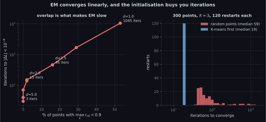
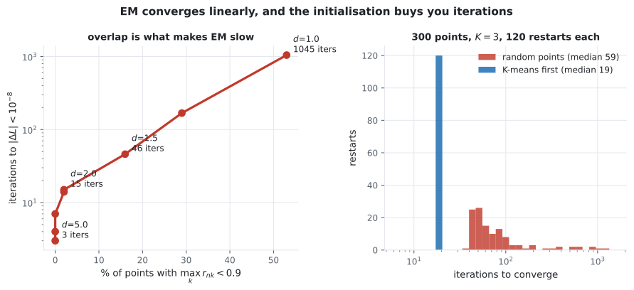
A factor of $348$ between the two ends, on data that differs only in how far apart the clusters are. That is the practical meaning of “linear convergence with a problem-dependent rate”: when the responsibilities are near $0.5$, each E-step barely moves them, so each M-step barely moves the parameters.

What the initialisation buys

$300$ points from three clusters, $K = 3$, $200$ restarts of each strategy:

initialisation	median iterations	mean iterations	share reaching the best optimum
random data points	$58$	$128.6$	$96.0\%$
K-means first	$\mathbf{19}$	$\mathbf{19.0}$	$\mathbf{100\%}$

The mean and median coincide for the K-means start, which is the interesting part: the long tail is gone entirely. Random starts occasionally land in a basin that takes hundreds of iterations to crawl out of; the K-means start never does, on this data.

This is why §11.5 points at K-means in the same breath as the GMM, and why every library implementation defaults to a K-means or K-means++ initialisation. It costs a few cheap iterations and removes both the worst case and the failures.

But it does not fix the real problem

Both strategies find the same best optimum, $-702.671823$. K-means makes EM reach it more often and faster — it does not make the optimum global.

Page 1102 measured the limit of what any initialisation can do: on seven points, $54.5\%$ of random starts collapse a component onto a data point, and those report a higher likelihood than any honest fit. No starting strategy can outrun an unbounded objective; that needs a variance floor or a prior, which §11.5 recommends and Bayesian PCA’s cousin — Bayesian GMM — supplies.

pch.quizTag Is EM clear?

1. What does the E-step compute, and what does the M-step do with it?

   A The E-step estimates the parameters and the M-step the responsibilities B The E-step computes the responsibilities from the current parameters; the M-step recomputes the parameters as three responsibility-weighted averages C Both compute the same thing D The E-step maximises and the M-step evaluates
   pch.quizShowAnswer

   B — The E-step computes the responsibilities from the current parameters; the M-step recomputes the parameters as three responsibility-weighted averages — Each half is easy given the other, and neither can be done first — that is the circularity page 1102 measured. EM alternates, and because each half exactly maximises a bound on the log-likelihood, the bound can never fall.

2. Over 180,000 EM steps, how often did the log-likelihood decrease?

   A Never B 11,163 times, but never by more than 8.9e-15 — the median decrease is exactly one unit in the last place C About half the time D Only when a component collapsed
   pch.quizShowAnswer

   B — 11,163 times, but never by more than 8.9e-15 — the median decrease is exactly one unit in the last place — Reporting this as 'never decreased' would be wrong. The honest statement is that no step decreased it by more than the rounding error of the quantity itself. The practical consequence: test new_L < old_L - tol, not new_L < old_L, or your convergence check will fire spuriously.

3. What sets how many iterations EM needs?

   A The number of data points B How much the components overlap — 1045 iterations when 53 percent of points are ambiguous, 3 when none are C The dimension D The number of components
   pch.quizShowAnswer

   B — How much the components overlap — 1045 iterations when 53 percent of points are ambiguous, 3 when none are — A factor of 348 between the two ends, on data differing only in cluster separation. When responsibilities sit near 0.5 the E-step barely moves them, so the M-step barely moves the parameters — that is linear convergence with a problem-dependent rate.

4. What does initialising with K-means buy?

   A A global optimum B Fewer iterations — median 19 against 58 — and it removes the long tail entirely, but the optimum it reaches is the same one C Nothing measurable D A different model
   pch.quizShowAnswer

   B — Fewer iterations — median 19 against 58 — and it removes the long tail entirely, but the optimum it reaches is the same one — Mean and median coincide at 19 for the K-means start, against a mean of 128.6 for random starts. Both find the same best value of -702.671823. No initialisation can outrun an unbounded objective — that needs a variance floor or a prior.

Exercises

Exercise 1 – Run Example 11.6 and define “converged”

pch.exerciseTag pch.exerciseTitle

Exercise 2 – How big are the decreases?

pch.exerciseTag pch.exerciseTitle

Exercise 3 – Overlap is what makes it slow

pch.exerciseTag pch.exerciseTitle

Exercise 4 – What K-means buys you

pch.exerciseTag pch.exerciseTitle

Recall card

• EM breaks a circular problem by refusing to solve both halves at once: fix the parameters and the responsibilities are a formula; fix the responsibilities and the parameters are three weighted averages.
• The E-step is Equation 11.53, the responsibilities. The M-step is Equations 11.54 to 11.56, in that order, each using what the step before produced.
• Example 11.6’s ‘after five iterations’ is the 1e-06 log-likelihood criterion, reproduced exactly; at 1e-09 it takes eight.
• The log-likelihood settles before the parameters do, at every tolerance, because it is flat near an optimum. Five against eleven at 1e-06.
• Neal and Hinton’s guarantee, measured over 180,000 steps: 11,163 register a negative change and none is larger than 8.9e-15.
• The median decrease is 1.776e-15, exactly one unit in the last place of a log-likelihood near minus fourteen. The theorem is about real numbers; this is what checking it in float64 looks like.
• So a convergence test should compare against a tolerance, not against zero, or it will fire spuriously.
• EM converges linearly, and overlap sets the rate: 1045 iterations when 53 percent of points are ambiguous, 3 when none are — a factor of 348.
• When responsibilities sit near one half the E-step barely moves them, so the M-step barely moves the parameters.
• A K-means initialisation cuts the median from 58 iterations to 19 and makes mean and median coincide — the long tail disappears.
• It also takes the share of runs reaching the best optimum from 96 to 100 percent, which is why every library implementation defaults to it.
• But it does not make the optimum global. No initialisation can outrun an unbounded objective; that needs a variance floor or a prior.

Next: The Latent Variable Perspective — §11.4, which explains where the responsibilities come from and why EM is the algorithm it is.