Regularization & Dropout

Regularisation is any pressure that stops a model fitting its training set perfectly. There are four common kinds, they work by completely different mechanisms, and one of them is routinely mis-measured because Keras reports a number that is not what you think it is. All four are measured below on the same over-parameterised network.

What you’ll learn

• Inverted dropout implemented by hand — and why Keras scales up during training rather than down at inference.
• The simplest regulariser measured: 13,002 parameters reached 0.8407 against 669,706 parameters’ 0.8467.
• Four dropout rates, where 0.5 was best and 0.7 began to underfit — with the train/validation gap moving from +0.1133 to −0.0090.
• Why Keras’ val_loss cannot be compared across L2 strengths, and what the plain cross-entropy shows instead: 0.6253 → 0.4810.
• L2’s actual effect on the weights: mean |w| falling 16× while the largest single weight grew.
• MC dropout: an accuracy gain inside the noise, but a spread 2.3× larger on wrong predictions.
• Max-norm, measured as a hard cap: 0 of 512 columns above the limit against 512 of 512 without it.

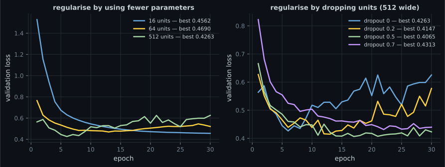
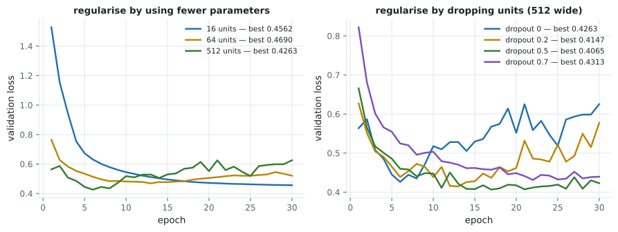
The cheapest regulariser is a smaller model

Before any penalty or noise, there is capacity. Two hidden layers on 6,000 Fashion-MNIST rows, Adam, 30 epochs:

figure Two ways to regularise the same problem matplotlib

Left: the 512-unit model reaches the lowest validation loss of the three (0.4263) and then throws it away, ending at 0.6253. The 16-unit model never overfits — it is still improving at epoch 30 — but it never gets as low either. Right: dropout 0.5 on the wide model reaches 0.4065, better than any width, and its curve barely rises afterwards.

Hidden width	Parameters	Best val loss	At epoch	Final val loss	Val accuracy
16	13,002	0.4562	30	0.4562	0.8407
64	55,050	0.4690	13	0.5210	0.8453
512	669,706	0.4263	6	0.6253	0.8467

Fifty times the parameters bought 0.0060 accuracy. The small model’s best and final losses are the same number, because it has no capacity to overfit with — which is a form of regularisation you get for free, along with a model that trains faster and ships smaller.

The wide model is not useless: it reaches a lower minimum. It just cannot stay there, which is what every other technique on this page is for.

Dropout

At each training step, zero each unit independently with probability $r$, then scale the survivors by $1/(1-r)$ so the layer’s expected output is unchanged:

$$\tilde{a}_i = \begin{cases} 0 & \text{with probability } r \\[2pt] \dfrac{a_i}{1-r} & \text{otherwise} \end{cases}$$

This is inverted dropout, and the scaling is why prediction needs no correction at all — the training-time output already has the right expectation. Measured on a matrix of ones with $r = 0.5$: the surviving entries all come out as exactly 2.0, and training=False returns the input unchanged.

Dropout rate	Best val loss	At epoch	Final val loss	Val accuracy	Train accuracy	Gap
0.0	0.4263	6	0.6253	0.8467	0.9600	0.1133
0.2	0.4147	13	0.5774	0.8453	0.9397	0.0944
0.5	0.4065	17	0.4230	0.8633	0.8930	0.0297
0.7	0.4313	22	0.4396	0.8533	0.8443	−0.0090

Three things happen as the rate rises. The overfitting turn moves later (epoch 6 → 13 → 17 → 22), the gap closes (0.1133 → −0.0090), and the training accuracy falls (0.9600 → 0.8443). At 0.7 the training accuracy is below the validation accuracy, which is the signature of a model being held back rather than generalised.

Dropout 0.5 was the best single result on this page: 0.8633 accuracy and a validation loss that ends 0.0165 above its own minimum, against the unregularised model’s 0.1990 above.

Dropout goes after the activation

keras.layers.Dense(512, activation="relu"),
keras.layers.Dropout(0.5),
keras.layers.Dense(512, activation="relu"),
keras.layers.Dropout(0.5),

diagram Diagram mermaid

  flowchart TD
  A["model overfits"] --> B{"can you use
a smaller model?"}
  B -- yes --> C["fewer units or layers
free, faster, smaller"]
  B -- "no: capacity is needed" --> D["dropout 0.2 to 0.5
strongest single lever here"]
  D --> E{"still overfitting?"}
  E -- yes --> F["add L2, and/or
get more data"]
  E -- no --> G["stop: check the gap
is not negative"]
  H["need uncertainty, not accuracy?"] --> I["keep dropout on at predict time
and average N passes"]

L2, and a measurement trap

$$L_{\text{total}} = L_{\text{data}} + \lambda \sum_i w_i^2$$

The gradient of that penalty is $2\lambda w$, so every step shrinks each weight in proportion to its own size — which is why L2 is also called weight decay.

The trap: Keras adds the penalty term to the loss it reports, including val_loss. Comparing val_loss across different $\lambda$ values therefore compares different quantities, and the stronger penalty looks worse purely because its own penalty is included. Measured both ways:

L2 $\lambda$	Keras val_loss	Plain cross-entropy	Val accuracy	mean |w|	max |w|
none	0.6253	0.6253	0.8467	0.0461	0.6245
1e−5	0.7049	0.6868	0.8413	0.0393	0.6833
1e−4	0.6451	0.5519	0.8560	0.0271	0.9342
1e−3	0.6913	0.5251	0.8133	0.0098	0.9499
1e−2	0.6469	0.4810	0.8360	0.0028	1.1726

Read the two loss columns against each other. On Keras’ number, L2 looks useless — every setting is worse than none. On the plain cross-entropy the strongest penalty is the best by a wide margin, 0.4810 against 0.6253. Same runs, opposite conclusions, and only one of the two columns is measuring what you meant.

Accuracy tells a third story, peaking at 1e−4 (0.8560) and dipping at 1e−3 (0.8133). With a 1,500-row validation set those swings are not reliable either. The one column that moves cleanly and monotonically is the mechanism:

figure What the penalty buys, and what it does matplotlib

Left uses validation accuracy rather than Keras' val_loss, because val_loss includes the penalty term and is not comparable across strengths. Right shows the actual effect: at 1e-2 the mean absolute weight is 0.0028 against 0.0461 with no penalty — a 16x reduction — while the largest single weight grows from 0.6245 to 1.1726. L2 penalises the sum of squares, so it flattens the bulk and tolerates a few large survivors.

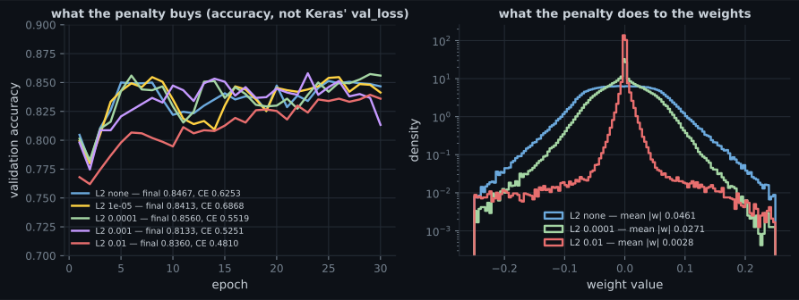
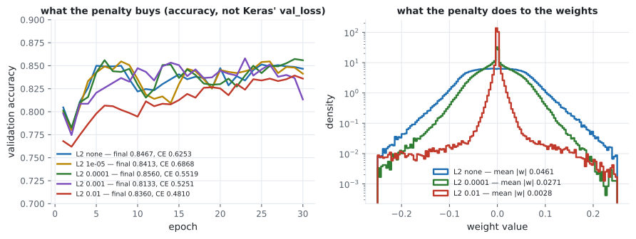
That last point is worth keeping. L2 does not bound any individual weight. It minimises the total sum of squares, and the cheapest way to do that is to crush the many small weights while letting a few genuinely useful ones grow. If you need a per-weight bound, that is what max-norm is for.

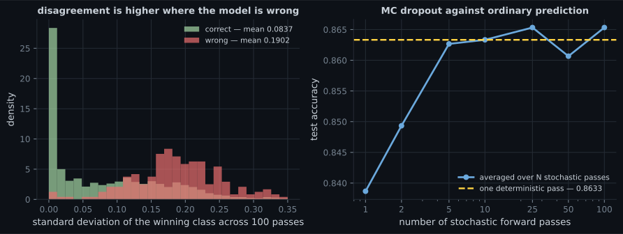
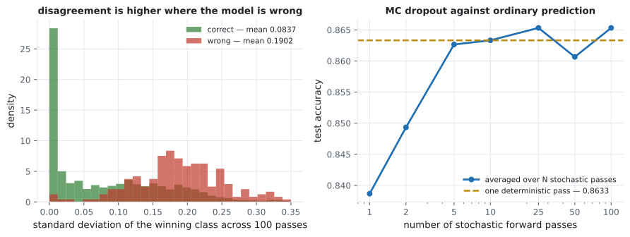
MC dropout: keeping the noise on at prediction time

Dropout is normally switched off for prediction. Leave it on, run the same input through the model 100 times, and you get a distribution instead of a point:

figure 100 stochastic passes over the same test set matplotlib

Left: on predictions the model got right the spread across passes averages 0.0837; on predictions it got wrong, 0.1902 — 2.3x wider. That separation is the useful output. Right: averaging the passes reaches 0.8653 against the deterministic 0.8633, a gain of 0.0020, and it is not even monotonic — 50 passes scored 0.8607. The accuracy benefit here is noise.

Passes averaged	Test accuracy
1 (stochastic)	0.8387
2	0.8493
5	0.8627
10	0.8633
25	0.8653
50	0.8607
100	0.8653
one deterministic pass	0.8633

The honest reading has two halves. The accuracy gain is not real: 0.8653 against 0.8633 is 0.0020 on a 1,500-row test set, and the non-monotonic 50-pass result confirms it is noise. The uncertainty signal is real: spread 0.0837 when correct against 0.1902 when wrong is a factor of 2.3, and it costs 100 forward passes to obtain.

If you need to know which predictions to distrust — for routing to a human, for abstention, for flagging out-of-distribution inputs — that spread is a usable signal, and MC dropout is the cheapest way to get one out of a model you have already trained. If you just want accuracy, spend the 100 passes elsewhere.

training=True is the whole trick

samples = np.stack([model(x_test, training=True).numpy() for _ in range(100)])
mean = samples.mean(axis=0)          # the averaged prediction
spread = samples.std(axis=0)         # how much the passes disagreed

sketch Dropout, one batch at a time p5.js Pause Restart

A layer of 24 units with a dropout mask applied. Drag the rate, press Resample to draw a new mask, and watch the survivors scale up by 1/(1-rate) so the sum stays put.

Max-norm: a hard cap instead of a penalty

Applied after every update, not added to the loss

keras.layers.Dense(512, activation="relu",
                   kernel_constraint=keras.constraints.MaxNorm(1.0, axis=0))

After each optimiser step, any column of the kernel whose norm exceeds the limit is rescaled down to it. Measured after five epochs:

	Max column norm	Mean column norm	Columns above 1.0
MaxNorm(1.0)	1.000001	0.999975	0 of 512
unconstrained	1.398920	1.191048	512 of 512

Every column sits exactly at the cap. That is the difference between a constraint and a penalty: L2 encourages small weights and lets exceptions through (max |w| grew to 1.1726 above), while max-norm forbids large ones. It pairs well with dropout and with high learning rates, because it makes a single oversized update harmless.

sketch The measured table, ranked p5.js Pause Restart

Click a column to rank every row by it. The bars are that column's values and the highest and lowest are computed from the numbers, not written in.

Pitfalls

• Comparing val_loss across L2 strengths. Keras includes the penalty in the reported loss. Compare accuracy, or recompute the plain cross-entropy.
• Adding dropout to a model that is not overfitting. At rate 0.7 the training accuracy fell below the validation accuracy — the model was being held back.
• Reaching for regularisation before trying a smaller model. 13,002 parameters got within 0.0060 of 669,706 here, and trained faster.
• Expecting L2 to bound individual weights. It minimises a sum, so a few weights grew while the mean fell 16×. Use MaxNorm for a real bound.
• Believing MC dropout improves accuracy. Measured gain 0.0020, non-monotonic across pass counts. Its value is the spread, not the mean.
• Forgetting training=True for MC dropout. model.predict disables dropout, so all 100 passes return the same numbers.
• Stacking every regulariser at once. Each one shifts the optimal setting of the others; add them one at a time and measure.
• Putting dropout before the activation. Convention and the measurements here put it after; zeroing pre-activations interacts badly with a following normalisation layer.

Recap

• Capacity is the first regulariser: 13,002 parameters reached 0.8407 against 669,706 parameters’ 0.8467, and never overfit.
• Inverted dropout scales survivors by $1/(1-r)$ during training, so inference needs no correction — verified as an exact ×2 at rate 0.5.
• Across rates 0.0 to 0.7, dropout moved the overfitting turn from epoch 6 to 22 and the train/validation gap from 0.1133 to −0.0090. Rate 0.5 was best at 0.8633.
• Keras’ val_loss includes the L2 penalty, which inverts the apparent ranking; on plain cross-entropy L2 improved the result from 0.6253 to 0.4810.
• L2 cut the mean absolute weight 16× while the largest weight grew — it bounds a sum, not any single weight.
• MC dropout’s accuracy gain was 0.0020 and non-monotonic; its spread separated correct from wrong predictions by a factor of 2.3.
• MaxNorm is a hard cap applied after every update: 0 of 512 columns exceeded it against 512 of 512 unconstrained.

Next

Seven techniques, each measured in isolation. The question that remains is the order to apply them in on a problem you have never seen: The Universal Workflow of Machine Learning.

pch.quizTag pch.quizDefaultTitle

1. Keras reported val_loss 0.6469 for L2 = 1e-2 and 0.6253 for no penalty, but the plain cross-entropy was 0.4810 against 0.6253. What explains the contradiction?

   A The plain cross-entropy was computed on different data B Keras adds the regularisation term to the loss it reports, so val_loss for a penalised model includes its own penalty — the two columns are not the same quantity C val_loss is computed before the final epoch's update D The model with L2 was still improving
   pch.quizShowAnswer

   B — Keras adds the regularisation term to the loss it reports, so val_loss for a penalised model includes its own penalty — the two columns are not the same quantity — Compare accuracy, or recompute the plain loss from the predictions. Comparing raw val_loss across penalty strengths is a category error.

2. At dropout 0.7 the training accuracy was 0.8443 and the validation accuracy 0.8533 — a negative gap. What does that indicate?

   A The validation set is easier than the training set B The regularisation is now strong enough to hold the model back on the training data itself, which is underfitting rather than generalisation C There is a bug in the evaluation code D Dropout is behaving correctly and this is the target state
   pch.quizShowAnswer

   B — The regularisation is now strong enough to hold the model back on the training data itself, which is underfitting rather than generalisation — A small positive gap is healthy. A negative one means the noise injected during training is costing more than the overfitting it prevents.

3. Why does inverted dropout scale the surviving units by 1/(1-r) during training?

   A To keep the gradients from vanishing B So the layer's expected output matches what it would be with no dropout — which means prediction needs no correction at all C To compensate for the reduced number of parameters D Because the loss function requires normalised inputs
   pch.quizShowAnswer

   B — So the layer's expected output matches what it would be with no dropout — which means prediction needs no correction at all — Verified: at rate 0.5 the survivors come out as exactly 2.0, and training=False returns the input unchanged.

4. MC dropout scored 0.8653 across 100 passes against 0.8633 for a single deterministic pass, but 0.8607 at 50 passes. What should you take from it?

   A 100 passes is the right number to use B The accuracy differences are noise; the genuinely useful output is the spread across passes, which was 2.3x larger on wrong predictions than on correct ones C MC dropout does not work with this architecture D The model needs more dropout
   pch.quizShowAnswer

   B — The accuracy differences are noise; the genuinely useful output is the spread across passes, which was 2.3x larger on wrong predictions than on correct ones — A non-monotonic sequence across pass counts is the giveaway. Use MC dropout when you need calibrated disagreement, not for a fraction of a point of accuracy.

5. L2 at 1e-2 reduced the mean absolute weight to 0.0028 while the largest single weight grew to 1.1726. Why?

   A The measurement is wrong — L2 shrinks every weight B L2 minimises the sum of squares, so the cheapest way to satisfy it is to crush the many small weights while letting a few genuinely useful ones grow C The largest weight belongs to a layer without the regulariser D Adam's adaptive scaling cancels the penalty for large weights
   pch.quizShowAnswer

   B — L2 minimises the sum of squares, so the cheapest way to satisfy it is to crush the many small weights while letting a few genuinely useful ones grow — If you need a bound on individual weights, MaxNorm gives one: 0 of 512 columns exceeded the cap, against 512 of 512 unconstrained.

🧪 Try It Yourself

pch.exerciseTag pch.exerciseTitle

pch.exerciseTag pch.exerciseTitle

pch.exerciseTag pch.exerciseTitle

pch.exerciseTag pch.exerciseTitle

pch.exerciseTag pch.exerciseTitle

pch.exerciseTag pch.exerciseTitle