First Example: Predicting House Prices (Regression)

404 training rows. That number governs this entire page. It is small enough that a single train/validation split is close to worthless — the four folds measured below disagree by 0.8018 MAE, which is a third of the score itself — and small enough that the model’s honest limitations are visible in a scatter plot rather than buried in aggregate statistics.

What you’ll learn

Why a regression head has no activation, and what happens to the loss if you add one.
MSE against MAE: which to train with, which to report, and the exact contribution one outlier makes to each.
Feature scaling with training statistics only, and the measured cost of skipping it: MAE 5.1459 against 2.6112.
K-fold validation on 404 rows, where the four folds report 1.8332, 2.3717, 2.6349 and 2.3216.
Two baselines: predicting the training median gives MAE 6.6608; the model gives 2.6112, a 60.8% improvement.
What the residuals show that MAE cannot: a +28.08 worst case, and systematic under-prediction of expensive houses.

The data

404 rows, 13 features, one continuous target

from tensorflow import keras
import numpy as np
 
(x_train, y_train), (x_test, y_test) = keras.datasets.boston_housing.load_data()
 
print(x_train.shape, x_test.shape)     # (404, 13) (102, 13)
print(y_train.min(), np.median(y_train), y_train.max())   # 5.0 20.8 50.0

The target is a median house price in thousands of dollars, ranging from 5.0 to 50.0. The 13 features are on wildly different scales:

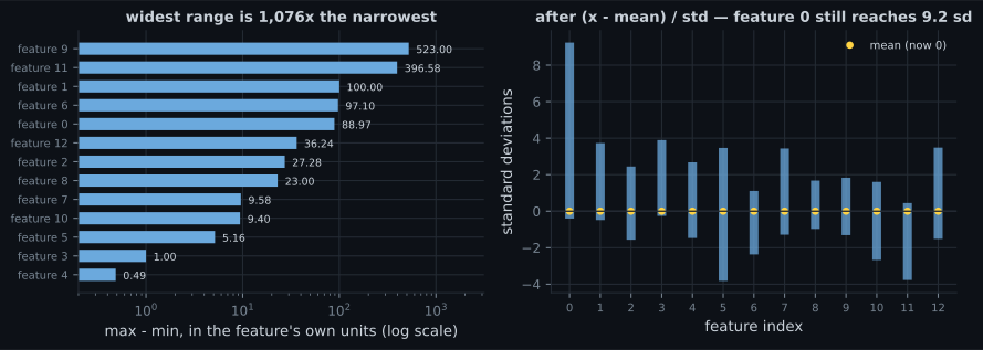
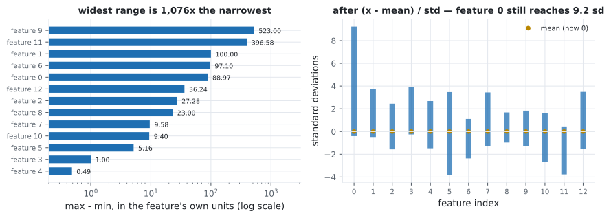
Two panels. Left: a horizontal bar chart of each feature's range width on a logarithmic axis, from 0.49 for the narrowest to 523.00 for the widest. Right: the same thirteen features after standardisation, drawn as vertical spans in standard deviations, all centred at zero but with feature 0 reaching above 9 standard deviations. — The widest feature spans 523.00 units and the narrowest 0.49 — a ratio of 1,076x. After subtracting the mean and dividing by the standard deviation every feature is centred at 0 with unit variance, but standardisation does not remove skew: feature 0 still reaches 9.2 standard deviations above its mean, because its distribution has a long right tail.

Standardise using the training mean and standard deviation, then apply that same transform to the test set:

Fit on train, transform both

mean = x_train.mean(axis=0)
std = x_train.std(axis=0)
x_train_scaled = (x_train - mean) / std
x_test_scaled = (x_test - mean) / std        # transformed, not re-fitted

The test set will not come out centred at zero — measured, its mean is +0.020827 and its standard deviation 0.983608. That is correct and expected. Fitting a scaler on the combined data shifts the feature means by up to 0.0303 standard deviations here, which is small but is still information from the test set leaking into training. The size of the leak is not the point; the habit is.

A regression head has no activation

The whole model

def build():
    model = keras.Sequential([
        keras.layers.Input((13,)),
        keras.layers.Dense(64, activation="relu"),
        keras.layers.Dense(64, activation="relu"),
        keras.layers.Dense(1),          # no activation
    ])
    model.compile("rmsprop", "mse", metrics=["mae"])
    return model

That bare Dense(1) is the only structural difference from the IMDB and Reuters models, and it matters:

Output layer	Range	Effect on this problem
`Dense(1)`	$(-\infty, \infty)$	correct — the target is 5.0 to 50.0
`Dense(1, activation="sigmoid")`	$(0, 1)$	can never exceed 1.0; every prediction is wrong by at least 4
`Dense(1, activation="relu")`	$[0, \infty)$	works, but any unit driven negative stops receiving gradient

diagram Diagram mermaid

  flowchart LR
  A["13 features
different units"] --> B["standardise
training mean and std"]
  B --> C["Dense 64 relu"]
  C --> D["Dense 64 relu"]
  D --> E["Dense 1
no activation"]
  E --> F["a price in $1000s"]
  G["train on MSE"] -.-> E
  H["report MAE"] -.-> F

MSE to train, MAE to report

\text{MSE} = \frac{1}{N}\sum_i (\hat{y}_i - y_i)^2 \qquad \text{MAE} = \frac{1}{N}\sum_i \lvert \hat{y}_i - y_i \rvert

They are not interchangeable. Take five errors, $[0.5, -0.5, 1.0, -1.0, 10.0]$ :

	Value	The single 10.0 error’s share
MAE	2.6000	0.7692
MSE	20.5000	0.9756

Squaring means MSE is dominated by the worst case — 97.6% of it comes from one of five errors. That makes MSE a good training signal, because its gradient grows with the error, so large mistakes are corrected first. MAE is the better report, because “off by 2.6” is in dollars a person understands, whereas “MSE 17.85” is in squared dollars.

The two losses also have different minimisers, which shows up in the baselines:

Constant prediction	Test MAE	Test MSE
training median (20.8)	6.6608	88.6654
training mean (22.4)	6.5330	83.7109

The median minimises absolute error, the mean minimises squared error — visible here as each baseline winning exactly one column. Neither is a coincidence.

Validating on 404 rows

With 404 training rows, holding out 100 leaves 304 to learn from and a validation set small enough that its score is mostly noise. K-fold validation trains K times, each on a different K−1 folds:

Four folds, four models

k, scores = 4, []
size = len(x_train_scaled) // k
for fold in range(k):
    val_x = x_train_scaled[fold * size:(fold + 1) * size]
    val_y = y_train[fold * size:(fold + 1) * size]
    part_x = np.concatenate([x_train_scaled[:fold * size],
                             x_train_scaled[(fold + 1) * size:]])
    part_y = np.concatenate([y_train[:fold * size],
                             y_train[(fold + 1) * size:]])
    model = build()
    model.fit(part_x, part_y, epochs=80, batch_size=16, verbose=0)
    scores.append(model.evaluate(val_x, val_y, verbose=0)[1])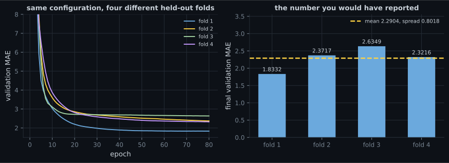

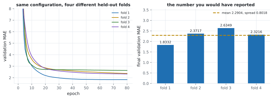
Two panels. Left: validation MAE against epoch for four folds, all falling steeply in the first ten epochs then flattening between 1.8 and 2.7 with the folds clearly separated. Right: a bar chart of each fold's final validation MAE — 1.83, 2.37, 2.63 and 2.32 — with a dashed line marking the mean of 2.29. — Nothing differs between these four runs except which 101 rows were held out. The results span 1.8332 to 2.6349 — a spread of 0.8018, which is 35% of the mean score of 2.2904. A single split would have reported any one of those four numbers as 'the' validation MAE.

Fold	Train rows	Validation rows	Validation MAE
1	303	101	1.8332
2	303	101	2.3717
3	303	101	2.6349
4	303	101	2.3216
mean			2.2904
spread			0.8018

If you had run one split and got fold 1, you would believe the model achieves 1.83. Run it again with a different split and you would believe 2.63 — a 44% difference in reported error from the same model and the same data. The spread is the finding, not the mean. On a dataset this small, report both.

Note also that all four folds reached their best validation MAE between epochs 70 and 80, so 80 epochs is not past the overfitting point here — unlike IMDB, where the turn came at epoch 4.

The final model, and what MAE hides

Train on everything, evaluate once

model = build()
model.fit(x_train_scaled, y_train, epochs=80, batch_size=16, verbose=0)
print(model.evaluate(x_test_scaled, y_test))
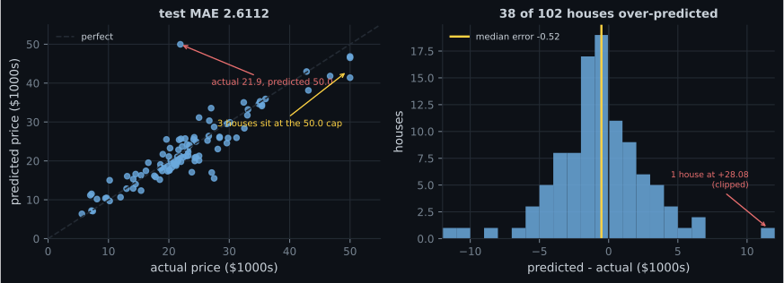
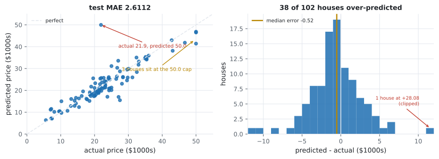
# test MSE 17.8460, test MAE 2.6112

MAE 2.6112 — about $2,611 off per house — against the median baseline’s 6.6608, a 60.8% improvement. That is the headline. The residuals are more informative:

Two panels. Left: predicted against actual price for 102 test houses, clustered along the diagonal, with three houses at the 50.0 target cap predicted well below it and one house of actual value 21.9 predicted at 50.0. Right: a histogram of residuals centred slightly left of zero, with one house clipped into the far right bin at plus 28. — The scatter tracks the diagonal closely in the 10-35 range and degrades at both ends. Three houses sit at the dataset's 50.0 target cap and are all under-predicted. One house with an actual value of 21.9 was predicted at 50.0 — a single error of +28.08, which is 43.3% of the total MSE but contributes only 0.28 of the 2.6112 MAE.

	Value
test MAE	2.6112
median residual	−0.5222
houses over-predicted	38 of 102
within $2,000	0.5490
within $5,000	0.8922
worst error	+28.08 (actual 21.9, predicted 50.0)
mean residual, houses ≥ 35.0 (n=10)	−2.6962
mean residual, houses < 35.0 (n=92)	−0.2081

Three things MAE alone would not have told you:

The model is biased low. 64 of 102 houses are under-predicted and the median residual is −0.52.
The bias is concentrated at the top. Expensive houses are under-predicted by 2.70 on average against 0.21 for the rest — partly because the target is capped at 50.0, so the training data contains no examples of what lies above it.
One catastrophic error exists. A house worth 21.9 was predicted at 50.0. If this were a pricing tool, that single output is the one that would matter, and no average over 102 houses will surface it.

What unscaled features cost

Everything identical, except the features go in raw:

Features	Test MSE	Test MAE
standardised	17.8460	2.6112
raw	47.4376	5.1459

Nearly twice the error, from four lines of preprocessing. The mechanism is the one derived on the gradient descent page: a weight’s gradient is proportional to its input, so a feature spanning 523 units generates gradients a thousand times larger than one spanning 0.49. A single learning rate has to satisfy the tightest axis, and every other weight then moves far too slowly.

sketch One learning rate, two feature scales p5.js

Gradient descent on a two-weight quadratic loss. Drag the scale slider to stretch one feature's range and watch the descent path go from a clean diagonal to a narrow zig-zag.

sketch The measured table, ranked p5.js

Click a column to rank every row by it. The bars are that column's values and the highest and lowest are computed from the numbers, not written in.

Pitfalls

Fitting the scaler on all the data. Use training statistics only. The test set should not come out perfectly centred, and that is the proof you did it right.
Putting an activation on the output. sigmoid caps predictions at 1.0 when the target reaches 50.0.
Reporting one train/validation split on a small dataset. Four folds here disagree by 0.8018 MAE. One split is a coin toss dressed as a measurement.
Reporting only the mean of the folds. The spread is the interesting number.
Confusing MSE and MAE units. MSE 17.85 is in squared thousands of dollars; its square root, 4.22, is comparable to the MAE of 2.61 and larger precisely because of the outlier.
Trusting an average error on 102 rows. The worst single error here is +28.08. Look at the residuals.
Ignoring a capped target. Prices stop at 50.0 in this dataset, so the model has never seen an example above it and systematically under-predicts the top of the range by 2.70.

Recap

Regression uses a Dense(1) output with no activation, MSE as the training loss, and MAE as the reported metric.
MSE is dominated by the worst error (97.6% of it from one of five errors in the worked example); MAE spreads blame evenly and is in interpretable units.
Standardise with training statistics only. Skipping it nearly doubled the error here, 5.1459 against 2.6112.
With 404 rows, K-fold is not optional: the four folds reported 1.8332 to 2.6349, a spread of 0.8018 around a mean of 2.2904.
The final model reaches MAE 2.6112 against the median baseline’s 6.6608 — a 60.8% improvement.
Residuals reveal what MAE hides: a low bias overall, a −2.70 bias on expensive houses caused by the 50.0 target cap, and one +28.08 catastrophe.

Phase 1 is complete: tensors, layers, activations, gradient descent, and three worked problems covering binary classification, multiclass classification and regression. Phase 2 takes on what happens when these networks get deep — the vanishing gradients, initialisation schemes, normalisation layers and regularisers that make depth trainable at all.

pch.quizTag pch.quizDefaultTitle

The four K-fold runs reported validation MAEs of 1.8332, 2.3717, 2.6349 and 2.3216. What is the most important thing that tells you?

pch.quizShowAnswer

B — With only 404 training rows, a single train/validation split would have reported any of those four numbers, so the spread of 0.8018 must be reported alongside the mean of 2.2904 — Nothing differed between the runs except which 101 rows were held out. A single-split score on data this small is mostly noise.
Why does the output layer use Dense(1) with no activation?

pch.quizShowAnswer

B — Because the target ranges from 5.0 to 50.0 and any squashing activation would restrict the output range — sigmoid, for instance, could never exceed 1.0 — The output has to be able to reach the target's range. ReLU would work here since prices are positive, but it adds a dead-unit failure mode for no benefit.
For the errors [0.5, -0.5, 1.0, -1.0, 10.0], the single 10.0 error contributes 97.6% of the MSE but only 76.9% of the MAE. What does that imply about which to use?

pch.quizShowAnswer

B — Train on MSE because its gradient grows with the error so large mistakes are corrected first, and report MAE because it is in the target's own units and easier to interpret — This is why Keras models here compile with loss='mse' and metrics=['mae'] — one number drives learning, the other communicates the result.
After scaling with training statistics, the test set has mean +0.020827 rather than exactly 0. Is that a bug?

pch.quizShowAnswer

B — No — the test set was transformed by the training mean and standard deviation, not fitted to its own, and a small offset is the expected consequence of doing it correctly — A test set that comes out perfectly centred is evidence the scaler saw it. Fitting on train+test here shifts feature means by up to 0.0303 standard deviations.
The model's mean residual is -2.6962 on houses priced at or above 35.0 versus -0.2081 below. What explains the difference?

pch.quizShowAnswer

B — The target is capped at 50.0, so the training data contains no examples above that ceiling and the model has no reason to predict near or beyond it — producing systematic under-prediction at the top — Three test houses sit exactly at 50.0 and all three are under-predicted. A censored target produces a censored model, and only a residual plot shows it.

🧪 Try It Yourself

pch.coffeeTagline

pch.coffeeCta

pch.feedbackHeading

pch.feedbackSubheading